Pricing the Future : Summary

[

Any book that promises a journey spanning 300 years is bound to focus on events that / people who made the maximum impact for the development of option pricing formula. If one were to pause and think about the option pricing formula, one would come up with questions like

• Pretty naïve question to start with, Why is there a need for options, in the first place? How were the traded historically? Were they precursor to some other instruments?

• What factors drive option prices? Can one mathematically pin down a few factors, assuming others are constant?

• Option by default depends on the movement of the underlying security. So , how to mathematically describe the underlying security?

  • Should one form an equation for the price?

  • Should one form an equation for price increments?

  • Should one assume a discrete process or a continuous process, after all traded price series is a discrete time series?

• Given a specific process for the underlying security, How does one go about figuring out the price of option?

This book in a way traces all the developments leading to Black Scholes equation like the Brownian motion, Ito’s calculus, Kolmogorov forward and backward equations,etc. and leading up to the most important idea of option prices, “replication”. Each of these ideas are described chapter wise. Let me summarize briefly, the chapters in this book.

Flowers and Spices

[

The book starts off describing Tulip mania of 1630’s and the reason it talks about Tulip mania is this : It was the first instance when government, in order to come out of a crisis, converted forward contracts to options contracts. The chapter then talks about Dutch East India company that dealt in Spices. The history of this company is closely linked to the emergence of the first formal market for options. Dutch East India company (VOC) became a powerful company in Netherlands just a few years from its inception. The shares of the company became valuable and a futures market emerged. Subsequently to cater to various kinds of demands, options market emerged for VOC shares. VOC finally got bogged down in corporate politics, corruption and became bankrupt. The period of 1680s was also the time when there was a need for communicating to general public about the ways to trade and understand options. To clarify the various terms and mechanics of options, Joseph de la Vega wrote extensively in his book,“Confusion of Confusions”. De la Vega was the first to describe in writing the workings of the stock market, in particular the trading of options. His work is held at such a high esteem that, since the year 2000, the federation of European Securities exchanges sponsor an annual prize for “outstanding research paper related to the securities markets in Europe”.

In the Beginning

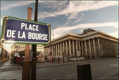
This chapter contains some important developments that happened in the financial markets between 1694 and 1885.The chapter starts off in 1694 with John Law advising French king on restoring the financial stability of the country. John Law started a firm in France that printed paper money. It was the first attempt in Europe to replace metal coins with paper money as legal tender. The bank, forerunner of France central bank, guaranteed that the notes would always be worth as much as the metal coins on which they were based. Law also convinced the king to grant him powers for a natural resource trading company so that he can bring in more revenues in to the country. Law’s company became very popular and there was a mad scramble amongst people to buy shares of the company. Like any bubble, the printing machine idea flopped by 1720 and France was facing an imminent financial disaster again. However the taste of trading and speculation activity that Law gave to French citizens was still in full force. Unofficial trading of various other instruments increased. So, finally in 1724, the government decided to bring some order in to this situation and an official Bourse was created. The whole system ran well until the French revolution in 1789 after which chaos ensued. There were few more developments that lead to the reopening of Paris Bourse and this time everybody was allowed to trade. Again forwards were outside the regulation but it did not stop the increasing volumes in the instruments and soon became the hub of speculators. Also with the collapse of a big investment bank, France went in to a recession. Out of all these developments, there was one positive development,legalization of forward market in 1885.

From Rags to Riches

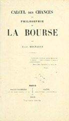
This chapter talks about the life of Jules Regnault. It is a classic rags to riches story. Why is the story relevant to the book or options pricing ? Well, Jules Regnault was the first person at least as per the book who deduced square root of time law. He not only tried proving it using math, but also used the law in the stock markets to retire rich. He started his work life at the age of 23 as a broker assistant. His living conditions were miserable but he managed to improve his living conditions by working hard in the broker’s office. Regnault was the first person to try to understand the workings of the stock exchange in mathematical terms, and his explanations had all the trappings of a scientific theory. Regnault managed this with hardly any formal education system. After a full day’s work at the Bourse, he would sit in a small room under the attic and do quant. Truly inspiring life. Remember this was in 1860s and he was investigating concepts such as random walks, role of information in stock markets, useful/harmful sides of speculation, insider information, factors that drive the valuation of an instrument, ways to calculate fair value of an instrument etc. An admirable quality about Jules Regnault’s life is that he never shied away from applying things in the stock market. He used all his principles at the Bourse and retired at the age of 47 after making a ton of money. In one sense, Jules Regnault can be called the first quant who made a fortune in the market.

**

The Banker’s Secretary

**

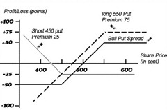
In any introductory book on options theory, you are likely to see payoff diagrams for various options and option strategies. This chapter talks about the first person to use these diagrams for communicating option positions, Henri Lefevre. Lefevre was a personal secretary to business tycoon James de Rothschild. Lefevre did not participate in speculation or trading activities but was a keen observer and educator of markets. He published various books and articles, thanks to the fact that he was a secretary to Rothschild and could influence the publishers. He made two main contributions to options theory. First contribution was his mental model of comparing economy and the flows of capital and goods with the human body and its organs. In Lefevre model of economy, stock exchange is like the heart that keeps blood moving through the veins, government is like a brain that thinks, combines and regulates the flow, Speculation is like the nervous system that provides the momentum that keeps commodities and capital in continuous motion. His second contribution was in 1873 and 1874 through his books. In those books he introduced a method of analysis that we are all familiar with, the pay off diagrams. The pay off diagrams for individual options might be very simple and a use of such a diagram to explain things could be a stretch. The real power of payoff diagrams comes in to play when you are analyzing a set of option positions. The final payoff diagram for a set of option positions, at once provides the price ranges where the entire position makes or loses money. Lefevre’s method and his extensive publications in the form of books , papers, articles, etc. helped the common masses understand options and options based investing in a better way.

The Spurned Professor

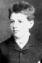
Louis Bachelier

The study of financial markets began in earnest at the turn of twentieth century. The first underpinnings of a mathematical theory were developed in the doctoral thesis of a thirty-year-old French student , Louis Bachelier. In 1900 Bachelier defended his PhD thesis and the committee composed on Poincare, Appell and Boussinesq awarded the thesis as “somewhat better than okay”. This evaluation haunted Bachelier through out his life as he could not secure a faculty position without a “real distinction” on his PhD. One of the reasons for Bachelier’s theory not getting attention was that it was incorrect. He analyzed price movements as a specific random walk ( an Arithmetic Brownian motion ) which allowed for stock prices to take negative values. So, the thesis that was probably the first step towards a mathematical treatment of financial markets lay dormant for a long time.

Botany, Physics and Chemistry

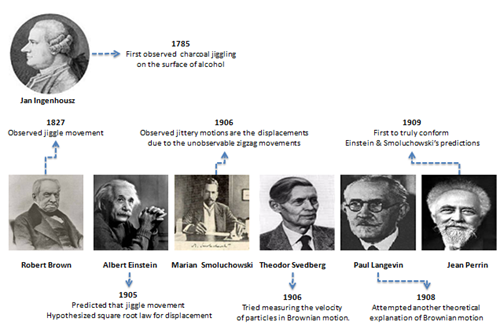
The first observation about the jiggle movement of particles was by a Dutch Scientist Jan Ingenhousz. However the credit goes to Robert Brown for the name. I find Robert Brown’s life very inspiring. He made use of his free time and did all the observations and work after work hours. He never socialized or dined out. Basically he was a guy who kept to himself and did outstanding work. He observed that Brownian motion never ceases though he never knew the reason for Brownian motion. Remember this was 1827 and molecular/atomic theory was not established. Then came along Einstein , aptly named as the father of atomic theory. He hypothesized and predicted the Brownian motion behavior. He also formulated the square root law by clarifying that one must not analyze a single drunkard’s walk but an ensemble of drunkard walks. In 1906 Marian Smoluchowski , another scientist made important contributions to understanding Brownian motion when he postulated that , the observed jittery motions are the displacements due to the unobservable zigzag movements that are a result of huge number of impacts. He concluded this after analyzing the speed of the particles at various resolutions. He saw that the velocity of the particles increased at higher resolutions. This made him conclude that whatever action that is seen in the microscope is basically the displacement. This book provides a fantastic analogy to Brownian motion which one will never forget after reading once. The books says it in a beautiful way:

Imagine the dance floor of a studio. Flashing strobe lights highlight the seemingly jerky movements of the dancers, Of course, even the coolest dancers do not disappear in to thin air between the flashes. They move contiguously through time and space, but their movements are hidden during the dark periods between flashes. In fact, there could be different dance steps that give rise to identical positions during the strobe flashes. This is the key point. Particles pushed around by the molecules in a liquid describe a continuous path, and the jerky motion we see under the microscope is just a sample of the entire movement.

In the next chapter, the book gives an account of Norbert Weiner’s life who proved that even for the jerkiest observations, it is practically certain that continuous paths exists which give rise to them. Typically these historical developments give so much meaning to what one gets to read on a pure mathematical text on Brownian motion. Brownian motion is continuous. “Oh! ok! ” was my first reaction when I studied stochastic calculus. However books such as these give so much context to mathematical properties that learning math becomes that much more interesting.

Disco Dancers and Strobe Lights

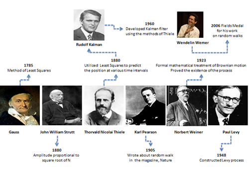
It was in 1880 that physicist John William Strutt discovered random walk in a completely different context, super imposition of waves of equal amplitudes, equal periods but random phases ? He came to the conclusion that amplitude was proportional to the square root of number of vibrations( variant of square root rule). Thorvald Nicolai Thiele, another scientist also worked on the random walk , while developing concepts in computational techniques. He used Gauss method of least square to conclude that an ensemble of particles following random walk would have an average displacement proportional to the square root of number of steps. Some 80 years later, this was picked up by another scientist Kalman and today we know a ton of applications of Kalman filter. Karl Pearson, the famous statistician added in a bit with his article in “Nature” magazine. Despite all these efforts, Brownian motion was not on sound mathematical foundation. It was Norbert Weiner who formally defined the process, proved its existence in a 40 page paper in 1923. In 1948, Paul Levy, considered as the founding father of probability theory , defined and constructed another class of random walks called Levy processes. In the last 60 years, more and more scientists studied various classes of random walks such as reflecting random walks, loop-erased random walks, biased random walks, random walks with drifts etc. In 2006, the prestigious Fields Medal, the Nobel prize equivalent in mathematics, was awarded to a French mathematician, Wendelin Werner, for his work on random walks.

The Overlooked Thesis

Regnault had brought Statistics , Lefevre Geometry and Bachelier Calculus to understanding options. This chapter highlights some of the important elements of Bachelier’s PhD thesis that shows how the thesis was so far removed from the traditional way of analyzing finance. The section mentions the following from the thesis

• The thesis referred to the efficient market hypothesis and formulates the mathematical equivalent of the same.

• It departs from the tradition of describing economic phenomenon verbally and uses mathematical equations to describe things.

• It showed that fluctuations of the stock price around true price follows Gaussian distribution.

• It showed two justifications for the square root of time law.

• It used Fourier methodology to derive heat equation in the context of price probabilities

• It showed that Options value depends on the security’s volatility and time

• It used reflecting principle to reduce the complexity involving Brownian motion calculations.

One of the offshoots of Bachelier thesis was Chapman-Kolmogorov equation that ties in the probability distribution of a variable at the end of a discrete Markov chain to its intermediate probabilities. Books such as these should be made required reading for a student before he/she gets exposed to math relating to Brownian motion. If you learn square root of time law using math and with no prior exposure to the rich history behind the development, you might learnt it but not appreciate the beauty that lies behind it. Similarly you might prove that Brownian path is nowhere differentiable but you will feel the result in a completely different way after reading Theoder Svedberg experiments about calculation of velocity of particles. All said and done, I strongly believe that historical developments about concepts/formulas are very important, sometimes more important than merely knowing a few ways to derivation of Black-Scholes equation.

Another Pioneer

Developments in science tend to be non-linear and controversy laden. Examples of plagiarism accusations are rampant. In such a context, it is but obvious that option pricing formula also has , in its history , some people whom we can only speculate that, they knew about a way to value options much before anyone else. One such individual mentioned in this chapter is Vincenz Bronzin. His work was accidentally discovered by Swiss historian Wolfgang Hafner, who later sent it to Prof Zimmermann. Both concluded that Vincenz Bronzin work in early 1920s had all the necessary math and concepts relating to pricing an option and in fact Bronzin’s work ends up deriving the same formula as Bachelier’s. The fact that his work was never popular/ recognized shows that historical development of any concept is tough to attribute to individuals. You never know that some person who never published stuff might have known the concept right through. Vincenz Bronzin work on option pricing was so advanced that some of the concepts looked similar to what the final Black-Scholes formula looked like, decades later.

Measuring the Immeasurable

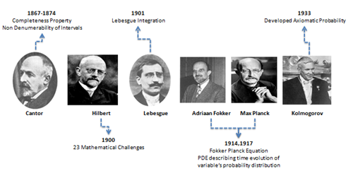
I loved this section where various historical figures are mentioned in the development of probability and stochastic processes. Firstly, what has a stochastic process got to do with pricing of options. What’s wrong with using / trying to use a deterministic process ? Well, the basic difference between a stochastic process and deterministic process is, in the latter case you can pin point the result and in the former case, you can only get a probability distribution for the result. So, all diffusion processes, arithmetic random walks and geometric random walks are all nothing but a way to summarize the particle movement and any computations on it will likely result in a probability distribution. Ok, let me get back to summarizing this chapter. This chapter talks about Kolmogorov, the father of modern probability. Picking on one of the Hilbert’s 23 problems that were announced in 1900, Kolmogorov developed a full-fledged axiomatic theory of probability in 1933. In doing so, he heavily relied on the works of Henri Lebesgue, George Cantor and Bachelier. Henri Lebesgue is credited for his revolutionary method of integration called the Lebesgue Integration that is applicable to a wide range of functions and sets of points. Lebesgue benefited from Cantor’s work on real line and introduced the concept of measure. Well , the development of Lebesgue integration is  in itself is a fantastic story and “The Calculus Gallery” covers it in a splendid way. Kolmogorov also derived Fokker Planck equation in his monograph, unaware that the PDE was developed in 1913 and 1914 by two physicists Adriaan Fokker and Max Planck to describe the time evolution of a variable’s probability distribution. The variable could be a particle’s position in a fluid or distribution of stock price. I liked this section because of a nice analogy that gives the difference between Chapman Kolmogorov and Fokker Planck equation. I love analogies as they are the first things that come to your mind than the raw equations. I paraphrase the author’s words here

The Chapman-Kolmogorov equation gives the probability of jumping from A to Z by investigating the probabilities for two consecutive jumps, say from A to P and then from P to Z, or from A to Q followed by a jump from Q to Z, and so on. It is like driving from New York in any direction and ending up in San Francisco. What are the chances of that happening ? Well, you could drive via Dallas, Texas, Via Witchita, Kansas, via Rapid City, South Dakota or via any other route. The probability of ending up in San Francisco is then computed by adding the probabilities of all possible routes. This is what the Chapman-Kolmogorov equation does. The Fokker-Planck equation goes one step further. It develops the whistle stop tours in to a distribution of probabilities of ending up anywhere on the West Coast, be it San Francisco, Santa Barabara, Los Angeles, or Tijuana, Mexico

After formulating the PDE, Kolmogorov found that the solution to the PDE was Chapman-Kolmogorov equation. He then turned the situation around: starting with a parabolic PDE, he pondered on the question whether it had a solution. If the answer was yes, then the solution could be none other than the Chapman-Kolmogorov equation. Thus he proved that Chapman-Kolmogorov equation indeed existed and was not merely a figment of imagination. Further development was needed in this area as there were strict conditions that one had to impose on Kolmogorov’s PDE describing Brownian motion so that it had a solution.

Accounting for Randomness

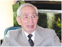
Kiyoshi Ito

This section talks about the contribution of Kiyoshi Ito. Since the Brownian motion is jagged and jittery at any resolution, one can’t calculate the velocity of the particles, as Marian Smoluchowski concluded in 1905. So how does one go about analyzing any Brownian path if the usual Riemann and Lebesgue Calculus cannot be applied ? Karl Weierstrass was the first mathematician who came up with such a nowhere differentiable function. How does one work with such functions? There is no way to slice the paths and handle it in the usual way. Whatever slice you look at , there will be jaggedness. What’s the way out? Here is where Ito comes in. In 1942 Ito published a paper that contained the mathematical machinery to handle such functions or paths. He used Taylor series expansion and found that the first three terms of the expansion were all that mattered for a stochastic process and thus ignored the rest to come up a forecast of probability distributions. Today Ito’s calculus is synonymous with “framework for handling Stochastic Differential equations”. Ito lived for 93 years and contributed immensely to field of Stochastics. In his Kyoto-Prize address, he says that he devised stochastic differential equations, after painstaking , solitary endeavors. For those who think that Solitude drives people crazy and must be avoided, Ito is a classic example of the tremendous possibilities of Solitude in life.

The Sealed Envelope

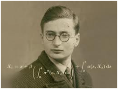
Wolfgang Doblin

This section talks about Wolfgang Doblin, a young mathematician who commits suicide while serving in the army to avoid getting killed by Germans. Before his death, he sends a sealed envelope to Academy of Paris. There is a big history behind the sealed envelopes that one can read from this section. The sealed envelope was supposed to be opened in 2040 but thankfully it gets opened in 2000. The math that Doblin sent to the academy had a framework to deal with Stochastic PDEs in such a way that one could lessen the restrictions imposed on it. Mathematicians wonder that if Doblin had not served in the army and had not met the fatal outcome, option pricing would have developed much earlier. In any case, a reader gets a glimpse in to this young genius,thanks to this book. Doblin’s life revolved around math and it served as a way to get him out of his gloomy and depressing environment. Though he only had the rare hour to focus entirely on math, usually during the night shifts hidden away in the telephone station that he was guarding and that provided some heat, his preoccupation with mathematical problems alleviated the dreariness and kept him from falling in to depression In one of his letter to his professor he writes,

Fortunately, my mathematical work helps me fight despair. As I am not interested in alcohol, I do not have the luxury of getting drunk like others.

The Utility of Logarithms

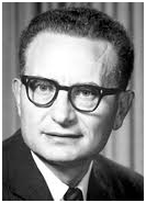
Paul Samuelson

This chapter talks about Paul Samuelson who relooked at Bachelier’s thesis and improvised on it. Instead of considering plain vanilla Brownian motion, Samuelson insisted on geometric brownian motion because of couple of reasons

• Share values are always positive in GBM scenario

• Price jumps, in percent, are equally distributed

• Model is in accordance with human nature, as displayed by Weber and Fechner’s psychology

• Data observed on stock exchanges fit GBM than Arithmetic Brownian motion

The chapter also mentions M.F.M.Osborne, a Physicist, who claimed in 1958, that log values and not the changes in stock prices are normally distributed. He was motivated to analyze the behavior after reading the works of psychologists Weber and Fechner. This observation is the same utility argument made by Daniel Bernoulli in 1713 while solving St.Petersburg Paradox.

The Nobelists -  The Three Musketeers

   [[

Fischer Black – Myron Scholes – Robert Merton

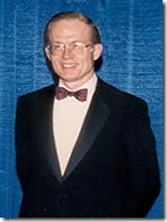
The next two chapters talk about Fischer Black, Myron Scholes and Robert Merton. MIT was one of the common denominators for all the three people. Fischer Black and Myron Scholes worked together on consulting projects for financial firms and thus were aware of markets and the places where quant techniques could be applied. They developed a good working rapport as Black’s forte was theory and Scholes was good at implementation. Robert Merton had worked on pricing warrants along with his MIT professor Samuelson. Warrants were similar to Options but for some technical differences. Before the trio cracked the formula, there were quite a number of scholars who came close to cracking it. In 1961, a graduate student in economics, Case Sprenkle made some headway. He assumed GBM for prices and allowed drift. But his approach was faulty as he posited that investor’s utility function would be revealed in prices. Also he ignored time value of money. In 1962, James Boness another student from Chicago also attempted and improvised on Sprenkle’s model by incorporating time value of money. However there were some problems with his theory as he assumed, all stocks on which the options are traded are defined to be of the same risk class and all investors are indifferent to risk. So, all attempts of Thorp, Case Sprenkle, James Boness, Robert Merton and Samuelson had shortcomings. But they all carried seeds of the eventual solution.

Somewhere in 1968 Fischer Black tried formulating the option price as PDE but faced a tough time solving the PDE. So, he filed it in his cabinet and went on with his work. However in 1969 , while conversing with his sole associate of his company, Myron Scholes, Black got a chance to start the work again. The key idea that was used in cracking the formula was “Portfolio hedging and replication” . If the option is deep in the money, then delta or the hedge ratio is 1. This means you can perfectly hedge a long call option by shorting one share of the underlying contract. If the option is not deep in the money but near ATM, then the hedge ratio is definitely not 1. It must be less than 1. If you represent the hedge ratio as x, then the combination of call and hedge position is basically a risk free portfolio growing at risk free rate. With the unknown hedge ratio as a variable, Black and Scholes wrote an equation describing option pricing.

With the PDE in hand, Black-Scholes made an educated guess that turned out to be the solution for option pricing formula. The solution to Black-Scholes PDE surprisingly did not have stock return component at all. This was totally unexpected from the prevailing notion that option price should somehow contain the return of the underlying instrument as one of its components. But Black-Scholes proved it otherwise. Robert Merton arrived at the same solution using Ito’s calculus. Initially Black had a lot of difficult publishing the paper in academic journals. It was only in 1973 that Black and Scholes managed to publish it under the title,”The Pricing of Options and Corporate Liabilities”, in Journal of Finance and Journal of Political Economy. According to a study undertaken in 2006, the paper garnered 2589 citations, making it the sixth most cited paper in all of economics. In the paper they acknowledged the fact that Merton had worked out a different approach and arrived at the same solution, thus kind of validating their final solution to option pricing.

The Higher They Climb …

This section highlights the lives of the three musketeers before the Nobel Prize award in recognition to the work. There are some people who believe that Texas Instruments was solely responsible for the tremendous marketing of Black Scholes formula by incorporating it in the module in its calculator. Traders did not need to know anything about the formula except the inputs. So, they happily traded away the options at CBOE that is today one of the biggest derivative exchanges in the world. Black joins Goldman at the age of 46 , becomes a partner with in two years and dies at the age of 56 (1995) because of cancer. Scholes and Merton land up at LTCM a fund using quant stuff to manage money. The principals get their recognition in the form of a Nobel Prize in 1997.

…The Harder They Fall

This section talks about the fall of LTCM. The LTCM bust is basically a `leverage' lesson for all money managers.If one needs to read in detail about the demise of LTCM, the book by Roger Lowenstein is spot on. This section does not fit the flow of the book.

The Long Tail

The last chapter talks about the problems behind Black-Scholes formula such as assuming volatility constant, assuming GBM that has normal distribution at it’s core. The books ends by saying

So, there are pitfalls and they can and do lead to spectacular failures like the LTCM crash, crisis of 2007, demise of Lehman Brothers. But to fault Black, Scholes and Merton and their equations for such aberrations would be utterly wrong. This would be like accusing Issac Newton and the laws of motion for fatal traffic accidents.

Takeaway

”What risk premium should be used for option pricing” was a stumbling block for developing the option pricing formula. The answers given by Black-Scholes-Merton surprised everyone : no risk premium at all. This book traces the historical developments leading to option pricing formula and in doing so, weaves an entertaining and a gripping narration of all the mathematical developments that were a precursor to Black-Scholes formula.