Decision Trees and Random Forests : A Visual Introduction For Beginners
This book provides a non-mathy entry point in to the world of decision trees and random forests.
Chapter 1 introduces the three kinds of learning algorithms:
-
Supervised Learning Algorithm: The algo feeds on labeled data and then use the fitted algorithm on unlabeled data
-
Unsupervised Learning Algorithm: The algo feeds on unlabeled data to figure out structure and patterns on its own
-
Semi-Supervised Learning: The algo feeds on labeled and unlabeled data. The algo needs to figure out the structure and patterns of the data. However it gets some help from the labeled data.
The algorithms covered in the book fall under Supervised learning category. Before understanding the decision tree, one needs to be familiar with the basic terminology. Chapter 2 of the book goes in to the meaning of various terms such as:
-
Decision Node
-
Chance Node
-
End Node
-
Root Node
-
Child Node
-
Splitting
-
Pruning
-
Branch
Chapter 3 goes in to creating a decision tree for a trivial example using pen and paper. In the process of doing so, it touches upon various aspects of the process, i.e. splitting, determining the purity of the node, determining the class label of a node etc. All of these are subtly introduced using plain English.
Chapter 4 talks about the three main strengths and weaknesses of hand-drawn decision trees.
Three main weaknesses:
-
Decision trees can change very quickly
-
Decision trees can become very complex
-
Decision trees can cause “paralysis by analysis”
Three main strengths:
-
Decision trees force you to consider outcomes and options
-
Decision trees help you visualize a problem
-
Decision trees help you prioritize
Decision Trees
Chapter 5 of the book gives a list of popular Decision tree algos. Decision tree can be used to perform two tasks: Classification and Regression, the former involves classifying cases based on certain features whereas the latter involves predicting a continuous value of a target variable based on input features. The five most common decision tree algos are,
-
ID3
-
C4.5
-
C5.0
-
CHAID
-
CART
Chapter 6 of the the book goes in to showcasing a simple dataset that contains movies watched by X based on certain attributes. The objective of the algo is to predict whether X will like a movie not present in the training sample, based on certain attributes. The first step in creating decision tree involves selecting the attribute based on which the root node needs to be split. The concept of “impurity” of a node is illustrated via a nice set of visuals.
Chapter 7 goes in to the math behind splitting the node, i.e using the principles of entropy and information gain. Once a node is split, one needs a metric to measure the purity of the node. This is done via entropy. For each split of an attribute, one can compute the entropy of the subset of the nodes. To aggregate the purity measures of subsets, one needs to understand the concept of Information gain. In the context of node splitting, the information gain is computed by the difference of entropies between the parent and the weighted average entropy of the children. Again a set of rich visuals are used to explain every component in the entropy formula and information gain (Kullback-Leibler divergence).
Chapter 8 addresses common questions around Decision trees
-
How/When does the algo stop splitting?
-
Allow the tree to split until every subset is pure
-
Stop the split until every leaf subset is pure
-
Adopt a stopping method
-
Stop when a tree reaches a max number of levels
-
Stop when a minimum information-gain level is reached
-
Stop when a subset contains less than a defined number of data points
-
-
-
Are there other methods to measure impurity ?
- Gini’s coefficient
-
What is greedy algo ?
- greedy algo selects nodes to build a tree by making a choice that seems best in the moment and never looks back
-
What if the dataset has two identical examples ?
- These are usually the noisy observations. Either the dataset can be increased or observations could be labeled correctly
-
What if there are more than 2 classes ?
- Logic remains the same. Only the entropy formula differs
Chapter 9 talks about the potential problems with Decision trees and the ways to address them
-
Overfitting
-
Statistical significance tests can be be used to check the information gain is significant or not
-
Pruning a tree so that there nodes with sparse data or incorrect fits can be removed
-
-
Information gain bias
- Information Gain Ratio reduces the bias that information gain has towards attributes that have large number of subsets. It accomplishes this by taking in to consideration the size and number of branches for each attribute
Chapter 10 gives an overview of Decision Tree Algorithms. Algorithms differ in the way the following aspects are handled:
-
How does the algorithm determine what to split?
-
How does the algorithm measure purity?
-
How does the algorithm know when to stop splitting?
-
How does the algorithm prune?
Here is a list of popular Decision tree algos with their pros and cons:
-
ID3 Algorithm Iterative Dichotomiser 3, is the “grandfather” of decision tree algorithms and was developed in 1986 by Ross Quinlan, a machine learning researcher.
-
Pros:
-
Easy to implement.
-
Very straightforward.
-
There is plenty of documentation available to help with implementation and working through issues.
-
-
Cons:
-
Susceptible to overfitting
-
Does not naturally handle numerical data.
-
Is not able to work with missing values.
-
-
-
C4.5 algorithm is the successor to the ID3 algorithm and was invented in 1993 by Ross Quinlan. It makes use of many of the same elements as the ID3 but also has number of improvements and benefits.
-
Pros:
-
Can work with either a continuous or discrete dataset. This means it can be used for classification or regression and work with categorical or numerical data
-
Can work with incomplete data.
-
Solves “overfitting” by pruning and its use of the Gain Ratio.
-
-
Cons:
-
Constructs empty branches with zero values.
-
Tends to construct very large trees with many subsets.
-
Susceptible to overfitting.
-
-
-
CART was first developed in 1984 and a unique characteristic of it is that it can only construct binary trees. ID3, C4.5 and CHAID are all able to construct multiple splits.
-
Pros:
-
Can work with either a continuous or discrete dataset. This means it can be used for classification or regression.
-
Can work with incomplete data.
-
-
Cons:
-
It can only split on a single variable.
-
Susceptible to instability.
-
Splitting method is biased towards nodes with more distinct values.
-
Overall, the algorithm can be biased towards nodes with more missing values.
-
-
Chapter 11 gives a sample python code to build a decision tree via CART.
Random Forests
A random forest is a machine learning algorithm that makes use of multiple decision trees to predict a result, and this collection of trees is often called an ensemble. The basic idea of random forest is that a decision tree is built based on a random set of observations from the available dataset.
Chapter 12 gives pros and cons of random forest algo
-
Pros:
-
More accurate than a single decision tree
-
More stable than a single decision tree
-
Less susceptible to the negative impact of greedy search
-
-
Cons
-
More Difficult to comprehend and interpret
-
Computationally expensive
-
Pros and cons of Decision tree
-
Pros:
-
easier to understand and interpet
-
less computational power
-
-
Cons:
-
tend to overfit
-
affected by small changes
-
affected by greedy search
-
Chapter 13 describes the basic algo behind random forest, i.e three steps. The first step involves selecting a subset of data.This is followed up by selecting random set of attributes from the bootstrapped sample.Based on the selected attributes, a best split is made and is repeated until a stopping criteria is reached.
Chapter 14 describes the way in which random forest predicts the response for a test data. There are two methods described in this chapter,i.e predicting with majority vote and predicting with mean
Chapter 15 explains the way to testing random forest for its accuracy. The method entails computing O.O.B estimate(Out of Bag error estimate).The key idea is to create a map between a data point and all the trees in which that data point does not act as a training sample. Once the map is created, for every randomized decision tree, you can find a set of data points that have not been used to train it and hence can be used to test the relevant decision tree.
Chapter 16 goes in to the details of computing attribute importance. The output of such computation is a set of relative scores for all the attributes in the dataset. These scores can be used to pre-process the data - remove all the unwanted attributes and rerun the random forest.
Chapter 17 answers some of the common questions around random forests
-
How many trees go in to random forest ?
- A safe number to start is between 64 and 128 trees
-
When do I use random forest vs decision tree ?
-
If you are concerned with accuracy, go for random forest
-
If you are concerned with interpretability, go for decision tree
-
Chapter 18 gives a sample python code to build a random forest vis Scikit-Learn library
Here are some of the visuals from the book:
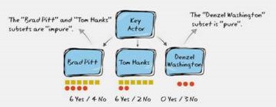
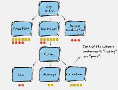

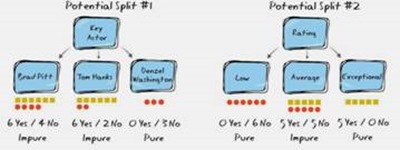
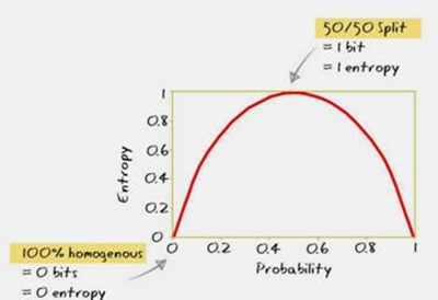
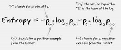

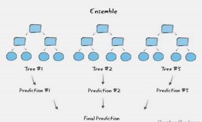
I think the visuals are the key takeaways from the book. You can read about the concepts mentioned in the book in a ton of places. However you might not find adequate visuals in a book that explains the math. This book is a quick read and might be worth your time as visuals serve as a power aid for learning and remembering concepts.