This blog post summarizes the book titled Data Manipulation in R, written by
Stephanie Locke.
The author clearly states that this book is for beginners. Well I would say that
even if you have good experience with R but have not worked with the recent
tidyverse package, then this book is worth the read. In any case, this book is
super short. An experienced R user can probably read it in a few hours.
Libraries used in the book
 1
 2
 3
 4
 5
 6
 7
 8
 9
10
11
| library(tidyverse)
library(ggplot2movies)
library(nycflights13)
library(odbc)
library(writexl)
library(openxlsx)
library(gapminder)
library(readr)
library(readxl)
library(lubridate)
library(stringr)
|
Getting Data
One can use readr , readxl and purr packages to efficiently read data from
multiple formats and combine them together.
1
2
3
4
5
6
7
8
| iris <- read_csv('./data/iris.csv')
iris <- iris%>%rename(Sepal.Length= sepal.length,
Sepal.Width = sepal.width,
Petal.Length = petal.length,
Petal.Width = petal.width,
Species = variety)
iris2 <- read_excel('./data/iris.xlsx')
iris3 <- map_df(list.files("./data/", pattern = "sample", full.names = TRUE), read_csv)
|
There are other packages being actively developed by R community that follow
the tidyverse philosophy.
Data Pipelines
This chapter introduced piping, an operator that allows us to create series of
connected transformations that goes from the source to the destination. Instead
of nesting functions you hook them together like pieces of plumbing so that your
data passes through them and changes as it goes.
The pipe operator was first designed and implemented in R by Stefan Milton
Bache in the package magrittr. Created in 2014, it is now very heavily used
and its widest option has been within the tidyverse.
1
2
3
4
| letters%>%toupper()%>%length()
## [1] 26
iris%>%head()%>%nrow()
## [1] 6
|
An interesting tidbit that I have learnt from the chapter is the assignment. I
have always used the assignment as follows
1
| temp <- iris %>% head()
|
But the author seems to be making a nice point where since the result of all the
operations are assigned to a variable, it is better to use RHS operator
1
| iris %>% head() -> temp
|
Whenever you use the functions with in a tidyverse framework, it is always
better to know the positional argument of data. By default, pipelines will put
our object as the first input to a function. To work with jumbled functions, we
need a way to tell our pipelines where to use our input instead of relying on
defaults. The way we can do that is with a period.
Filtering Columns
This chapter introduces a bunch of different ways to select features from a tibble
 1
 2
 3
 4
 5
 6
 7
 8
 9
10
11
12
13
14
15
16
17
18
19
20
21
22
23
24
25
26
27
28
29
30
31
32
33
34
35
36
37
38
39
40
41
42
43
44
45
46
|
iris%>%select(Species)%>%head(1)
## # A tibble: 1 x 1
##   Species
##   <chr>
## 1 Setosa
iris%>%select(-Species)%>%head(1)
## # A tibble: 1 x 4
##   Sepal.Length Sepal.Width Petal.Length Petal.Width
##          <dbl>       <dbl>        <dbl>       <dbl>
## 1          5.1         3.5          1.4         0.2
iris%>%select(Sepal.Length:Petal.Length)%>%head(1)
## # A tibble: 1 x 3
##   Sepal.Length Sepal.Width Petal.Length
##          <dbl>       <dbl>        <dbl>
## 1          5.1         3.5          1.4
iris%>%select(-(Sepal.Length:Petal.Length))%>%head(1)
## # A tibble: 1 x 2
##   Petal.Width Species
##         <dbl> <chr>
## 1         0.2 Setosa
iris%>%select(starts_with('s'))%>%head(1)
## # A tibble: 1 x 3
##   Sepal.Length Sepal.Width Species
##          <dbl>       <dbl> <chr>
## 1          5.1         3.5 Setosa
iris%>%select(ends_with('s'))%>%head(1)
## # A tibble: 1 x 1
##   Species
##   <chr>
## 1 Setosa
iris%>%select(contains('Length'))%>%head(1)
## # A tibble: 1 x 2
##   Sepal.Length Petal.Length
##          <dbl>        <dbl>
## 1          5.1          1.4
iris%>%select_if(is.numeric) %>%head(1)
## # A tibble: 1 x 4
##   Sepal.Length Sepal.Width Petal.Length Petal.Width
##          <dbl>       <dbl>        <dbl>       <dbl>
## 1          5.1         3.5          1.4         0.2
iris%>%select_if(~is.numeric(.) & n_distinct(.)>30) %>%head(1)
## # A tibble: 1 x 2
##   Sepal.Length Petal.Length
##          <dbl>        <dbl>
## 1          5.1          1.4
|
Filtering Rows
This chapter introduces basic syntax around using slice, filter_if ,
filter_all and filter_at functions.
 1
 2
 3
 4
 5
 6
 7
 8
 9
10
11
12
13
14
15
16
17
18
19
20
21
22
23
24
25
26
27
28
29
30
31
32
33
34
35
36
37
38
39
40
41
| iris%>%slice(1:2)
## # A tibble: 2 x 5
## Sepal.Length Sepal.Width Petal.Length Petal.Width Species
## <dbl> <dbl> <dbl> <dbl> <chr>
## 1 5.1 3.5 1.4 0.2 Setosa
## 2 4.9 3 1.4 0.2 Setosa
iris%>%filter(Species=='Virginica') %>% head(1)
## # A tibble: 1 x 5
## Sepal.Length Sepal.Width Petal.Length Petal.Width Species
## <dbl> <dbl> <dbl> <dbl> <chr>
## 1 6.3 3.3 6 2.5 Virginica
iris%>%filter(Species == 'Virginica', Sepal.Length > mean(Sepal.Length))%>%head(1)
## # A tibble: 1 x 5
## Sepal.Length Sepal.Width Petal.Length Petal.Width Species
## <dbl> <dbl> <dbl> <dbl> <chr>
## 1 6.3 3.3 6 2.5 Virginica
iris%>%filter(Species == 'Virginica'|Sepal.Length > mean(Sepal.Length))%>%head(1)
## # A tibble: 1 x 5
## Sepal.Length Sepal.Width Petal.Length Petal.Width Species
## <dbl> <dbl> <dbl> <dbl> <chr>
## 1 7 3.2 4.7 1.4 Versicolor
iris%>%filter_all(any_vars(.>7.5))%>%head(1)
## # A tibble: 1 x 5
## Sepal.Length Sepal.Width Petal.Length Petal.Width Species
## <dbl> <dbl> <dbl> <dbl> <chr>
## 1 5.1 3.5 1.4 0.2 Setosa
iris%>%select_if(is.numeric)%>%filter_all(any_vars(abs(. - mean(.) ) > 2*sd(.))) %>% head(1)
## # A tibble: 1 x 4
## Sepal.Length Sepal.Width Petal.Length Petal.Width
## <dbl> <dbl> <dbl> <dbl>
## 1 5.8 4 1.2 0.2
iris%>%filter_if(~is.numeric(.), any_vars(.<mean(.)))%>% head(1)
## # A tibble: 1 x 5
## Sepal.Length Sepal.Width Petal.Length Petal.Width Species
## <dbl> <dbl> <dbl> <dbl> <chr>
## 1 5.1 3.5 1.4 0.2 Setosa
iris%>%filter_at(vars(ends_with("Length")), any_vars(.<mean(.)))%>% head(1)
## # A tibble: 1 x 5
## Sepal.Length Sepal.Width Petal.Length Petal.Width Species
## <dbl> <dbl> <dbl> <dbl> <chr>
## 1 5.1 3.5 1.4 0.2 Setosa
|
Working with names
This chapter introduces some of the functions relating to renaming rows and
columns of a tibble
 1
 2
 3
 4
 5
 6
 7
 8
 9
10
11
12
13
14
15
16
17
18
| iris%>% select_all(str_to_lower)%>%head(1)
## # A tibble: 1 x 5
## sepal.length sepal.width petal.length petal.width species
## <dbl> <dbl> <dbl> <dbl> <chr>
## 1 5.1 3.5 1.4 0.2 Setosa
iris%>%rename_if(is.numeric, str_to_lower)%>% head(1)
## # A tibble: 1 x 5
## sepal.length sepal.width petal.length petal.width Species
## <dbl> <dbl> <dbl> <dbl> <chr>
## 1 5.1 3.5 1.4 0.2 Setosa
iris%>%rename_at(vars(starts_with('S')), str_to_lower) %>%head(1)
## # A tibble: 1 x 5
## sepal.length sepal.width Petal.Length Petal.Width species
## <dbl> <dbl> <dbl> <dbl> <chr>
## 1 5.1 3.5 1.4 0.2 Setosa
mtcars%>%rownames_to_column("cars") %>%head(1)
## cars mpg cyl disp hp drat wt qsec vs am gear carb
## 1 Mazda RX4 21 6 160 110 3.9 2.62 16.46 0 1 4 4
|
Re-arranging your data
The following snippets summarize the main syntax introduced in this chapter:
 1
 2
 3
 4
 5
 6
 7
 8
 9
10
11
12
13
14
15
16
17
18
19
20
21
22
23
24
25
26
27
28
29
30
31
32
33
34
35
36
37
38
| iris%>%arrange(desc(Species))%>%head(1)
## # A tibble: 1 x 5
## Sepal.Length Sepal.Width Petal.Length Petal.Width Species
## <dbl> <dbl> <dbl> <dbl> <chr>
## 1 6.3 3.3 6 2.5 Virginica
iris%>%arrange(desc(Species), Sepal.Length)%>%head(1)
## # A tibble: 1 x 5
## Sepal.Length Sepal.Width Petal.Length Petal.Width Species
## <dbl> <dbl> <dbl> <dbl> <chr>
## 1 4.9 2.5 4.5 1.7 Virginica
iris %>%
arrange_all() %>%
head(1)
## # A tibble: 1 x 5
## Sepal.Length Sepal.Width Petal.Length Petal.Width Species
## <dbl> <dbl> <dbl> <dbl> <chr>
## 1 4.3 3 1.1 0.1 Setosa
iris %>%
arrange_if(is.character, desc) %>%
head(1)
## # A tibble: 1 x 5
## Sepal.Length Sepal.Width Petal.Length Petal.Width Species
## <dbl> <dbl> <dbl> <dbl> <chr>
## 1 6.3 3.3 6 2.5 Virginica
iris %>%
arrange_at(vars(Species, starts_with('P')), desc) %>%
head(1)
## # A tibble: 1 x 5
## Sepal.Length Sepal.Width Petal.Length Petal.Width Species
## <dbl> <dbl> <dbl> <dbl> <chr>
## 1 7.7 2.6 6.9 2.3 Virginica
iris %>%
select(sort(tidyselect::peek_vars())) %>%
head(1)
## # A tibble: 1 x 5
## Petal.Length Petal.Width Sepal.Length Sepal.Width Species
## <dbl> <dbl> <dbl> <dbl> <chr>
## 1 1.4 0.2 5.1 3.5 Setosa
|
Changing your Data
The following snippets summarize the main syntax introduced in this chapter:
  1
  2
  3
  4
  5
  6
  7
  8
  9
 10
 11
 12
 13
 14
 15
 16
 17
 18
 19
 20
 21
 22
 23
 24
 25
 26
 27
 28
 29
 30
 31
 32
 33
 34
 35
 36
 37
 38
 39
 40
 41
 42
 43
 44
 45
 46
 47
 48
 49
 50
 51
 52
 53
 54
 55
 56
 57
 58
 59
 60
 61
 62
 63
 64
 65
 66
 67
 68
 69
 70
 71
 72
 73
 74
 75
 76
 77
 78
 79
 80
 81
 82
 83
 84
 85
 86
 87
 88
 89
 90
 91
 92
 93
 94
 95
 96
 97
 98
 99
100
101
102
103
104
105
106
107
108
109
110
111
112
113
114
115
116
| iris %>%
mutate(x = Sepal.Width * Sepal.Length) %>%
head(1)
## # A tibble: 1 x 6
## Sepal.Length Sepal.Width Petal.Length Petal.Width Species x
## <dbl> <dbl> <dbl> <dbl> <chr> <dbl>
## 1 5.1 3.5 1.4 0.2 Setosa 17.8
iris %>%
mutate(Sepal.Width=NULL) %>%
head(1)
## # A tibble: 1 x 4
## Sepal.Length Petal.Length Petal.Width Species
## <dbl> <dbl> <dbl> <chr>
## 1 5.1 1.4 0.2 Setosa
iris %>%
mutate(id = row_number()) %>%
head(1)
## # A tibble: 1 x 6
## Sepal.Length Sepal.Width Petal.Length Petal.Width Species id
## <dbl> <dbl> <dbl> <dbl> <chr> <int>
## 1 5.1 3.5 1.4 0.2 Setosa 1
iris %>%
mutate(size= case_when(
Sepal.Length<mean(Sepal.Length) ~ "s",
Sepal.Length>mean(Sepal.Length) ~ "l",
TRUE ~ "m"
)) %>%
head(1)
## # A tibble: 1 x 6
## Sepal.Length Sepal.Width Petal.Length Petal.Width Species size
## <dbl> <dbl> <dbl> <dbl> <chr> <chr>
## 1 5.1 3.5 1.4 0.2 Setosa s
iris %>%
mutate(Species = case_when(
Species == 'setosa' ~ toupper(Species),
TRUE ~ as.character(Species)
)) %>%
head(1)
## # A tibble: 1 x 5
## Sepal.Length Sepal.Width Petal.Length Petal.Width Species
## <dbl> <dbl> <dbl> <dbl> <chr>
## 1 5.1 3.5 1.4 0.2 Setosa
iris %>%
mutate(runagg = cumall(Sepal.Length < mean(Sepal.Length))) %>%
head(1)
## # A tibble: 1 x 6
## Sepal.Length Sepal.Width Petal.Length Petal.Width Species runagg
## <dbl> <dbl> <dbl> <dbl> <chr> <lgl>
## 1 5.1 3.5 1.4 0.2 Setosa TRUE
iris %>%
transmute(Sepal.Width = floor(Sepal.Width),
Species == case_when(
Species == 'setosa' ~ toupper(Species),
TRUE ~ as.character(Species))) %>%
head(1)
## # A tibble: 1 x 2
## Sepal.Width `==...`
## <dbl> <lgl>
## 1 3 TRUE
iris %>%
mutate_all(as.character)
## # A tibble: 150 x 5
## Sepal.Length Sepal.Width Petal.Length Petal.Width Species
## <chr> <chr> <chr> <chr> <chr>
## 1 5.1 3.5 1.4 0.2 Setosa
## 2 4.9 3 1.4 0.2 Setosa
## 3 4.7 3.2 1.3 0.2 Setosa
## 4 4.6 3.1 1.5 0.2 Setosa
## 5 5 3.6 1.4 0.2 Setosa
## 6 5.4 3.9 1.7 0.4 Setosa
## 7 4.6 3.4 1.4 0.3 Setosa
## 8 5 3.4 1.5 0.2 Setosa
## 9 4.4 2.9 1.4 0.2 Setosa
## 10 4.9 3.1 1.5 0.1 Setosa
## # ... with 140 more rows
iris %>%
mutate_if(is.numeric,~. +rnorm(.))
## # A tibble: 150 x 5
## Sepal.Length Sepal.Width Petal.Length Petal.Width Species
## <dbl> <dbl> <dbl> <dbl> <chr>
## 1 5.69 2.02 1.89 -0.526 Setosa
## 2 3.35 2.56 1.37 -0.285 Setosa
## 3 5.79 2.36 0.739 -0.134 Setosa
## 4 3.82 1.41 1.80 -1.20 Setosa
## 5 5.53 2.16 1.45 0.262 Setosa
## 6 4.57 4.17 -0.261 0.918 Setosa
## 7 5.63 2.62 1.65 0.697 Setosa
## 8 4.20 5.27 -0.121 -0.808 Setosa
## 9 2.40 3.58 0.253 0.0210 Setosa
## 10 5.14 4.42 0.695 -1.64 Setosa
## # ... with 140 more rows
iris %>%
mutate_at(vars(Sepal.Width:Petal.Width), ~ . +rnorm(.))
## # A tibble: 150 x 5
## Sepal.Length Sepal.Width Petal.Length Petal.Width Species
## <dbl> <dbl> <dbl> <dbl> <chr>
## 1 5.1 4.60 0.0330 -2.38 Setosa
## 2 4.9 2.82 0.946 2.72 Setosa
## 3 4.7 4.54 0.371 0.645 Setosa
## 4 4.6 4.00 1.16 1.39 Setosa
## 5 5 4.28 1.01 0.679 Setosa
## 6 5.4 1.55 1.70 -0.0684 Setosa
## 7 4.6 2.85 0.196 -0.0835 Setosa
## 8 5 3.59 0.379 -0.448 Setosa
## 9 4.4 1.64 1.65 0.848 Setosa
## 10 4.9 3.61 1.28 -0.817 Setosa
## # ... with 140 more rows
|
Working with dates and times
The following snippets summarize the main syntax introduced in this chapter:
relating to lubridate package
 1
 2
 3
 4
 5
 6
 7
 8
 9
10
11
12
13
14
15
16
17
18
19
20
21
22
23
24
25
26
27
28
29
30
| test_date <- ymd_hms("20210505140101")
yday(test_date);mday(test_date);wday(test_date);
## [1] 125
## [1] 5
## [1] 4
hour(test_date);minute(test_date);second(test_date)
## [1] 14
## [1] 1
## [1] 1
test_date + years(1)
## [1] "2022-05-05 14:01:01 UTC"
test_date + months(1)
## [1] "2021-06-05 14:01:01 UTC"
test_date + days(1)
## [1] "2021-05-06 14:01:01 UTC"
test_date + minutes(1)
## [1] "2021-05-05 14:02:01 UTC"
format(test_date, c("%Y","%F","%z"))
## [1] "2021" "2021-05-05" "+0000"
floor_date(test_date, "month");ceiling_date(test_date, 'month')
## [1] "2021-05-01 UTC"
## [1] "2021-06-01 UTC"
test_date + months(1:4)
## [1] "2021-06-05 14:01:01 UTC" "2021-07-05 14:01:01 UTC"
## [3] "2021-08-05 14:01:01 UTC" "2021-09-05 14:01:01 UTC"
test_date %m+% months(1:4)
## [1] "2021-06-05 14:01:01 UTC" "2021-07-05 14:01:01 UTC"
## [3] "2021-08-05 14:01:01 UTC" "2021-09-05 14:01:01 UTC"
test_date %within% interval(ymd('20190101'), ymd('20220101'))
## [1] TRUE
|
Working with text
The following snippets summarize the main syntax introduced in this chapter :
relating to stringr , purrr and forcats package
 1
 2
 3
 4
 5
 6
 7
 8
 9
10
11
12
13
14
15
16
17
18
19
20
21
22
23
24
25
26
27
28
29
30
31
32
33
34
35
36
37
38
39
40
41
42
43
44
45
46
47
48
49
50
51
52
53
| simple <- "This IS HOrribly typed! "
numbers <- c('02', '11', '10', '1')
str_detect(simple, 'typed')
## [1] TRUE
str_extract(simple, 'typed.*')
## [1] "typed! "
str_replace(simple, 'typed', 'written')
## [1] "This IS HOrribly written! "
str_replace_all(simple,'r', 'b')
## [1] "This IS HObbibly typed! "
str_count(simple, "[iI]")
## [1] 3
patterns <- c("[aeiou]","[aeiou].*$", "[a-z]", "^[A-Z]", "[:punct:]$", "r{2}", "[aeiou]b")
for( pat in patterns){
print(str_extract(simple,pat))
print(str_extract_all(simple,pat))
print(str_detect(simple,pat))
}
## [1] "i"
## [[1]]
## [1] "i" "i" "e"
##
## [1] TRUE
## [1] "is IS HOrribly typed! "
## [[1]]
## [1] "is IS HOrribly typed! "
##
## [1] TRUE
## [1] "h"
## [[1]]
## [1] "h" "i" "s" "r" "r" "i" "b" "l" "y" "t" "y" "p" "e" "d"
##
## [1] TRUE
## [1] "T"
## [[1]]
## [1] "T"
##
## [1] TRUE
## [1] NA
## [[1]]
## character(0)
##
## [1] FALSE
## [1] "rr"
## [[1]]
## [1] "rr"
##
## [1] TRUE
## [1] "ib"
## [[1]]
## [1] "ib"
##
## [1] TRUE
|
String Splitting
 1
 2
 3
 4
 5
 6
 7
 8
 9
10
11
12
13
14
15
16
| str_split(simple, "i")
## [[1]]
## [1] "Th" "s IS HOrr" "bly typed! "
str_split(simple, "[iI]")
## [[1]]
## [1] "Th" "s " "S HOrr" "bly typed! "
str_to_lower(simple); str_to_upper(simple); str_to_title(simple)
## [1] "this is horribly typed! "
## [1] "THIS IS HORRIBLY TYPED! "
## [1] "This Is Horribly Typed! "
str_trim(simple)
## [1] "This IS HOrribly typed!"
str_order(numbers, numeric=TRUE)
## [1] 4 1 3 2
str_length(numbers)
## [1] 2 2 2 1
|
Advanced operations
 1
 2
 3
 4
 5
 6
 7
 8
 9
10
11
12
13
14
15
16
17
| strings <- c("A word" , "Two words", "Not three words")
strings %>%
str_split(boundary("word")) %>%
str_detect("w")
## [1] TRUE TRUE TRUE
strings %>%
str_split(boundary("word")) %>%
map(str_detect,"w")
## [[1]]
## [1] FALSE TRUE
##
## [[2]]
## [1] TRUE TRUE
##
## [[3]]
## [1] FALSE FALSE TRUE
|
Factor operations
 1
 2
 3
 4
 5
 6
 7
 8
 9
10
11
12
13
14
15
16
17
18
19
20
21
22
23
24
| my_string <- c("red", "blue", "yellow", NA, "red")
fct_count(my_string)
## # A tibble: 4 x 2
## f n
## <fct> <int>
## 1 blue 1
## 2 red 2
## 3 yellow 1
## 4 <NA> 1
fct_explicit_na(my_string)
## [1] red blue yellow (Missing) red
## Levels: blue red yellow (Missing)
fct_infreq(my_string)
## [1] red blue yellow <NA> red
## Levels: red blue yellow
fct_lump(my_string, n =1)
## [1] red Other Other <NA> red
## Levels: red Other
fct_lump(my_string, prop=0.25, other_level = "OTHER")
## [1] red OTHER OTHER <NA> red
## Levels: red OTHER
fct_lump(my_string, n = -1, other_level = "other")
## [1] red blue yellow <NA> red
## Levels: blue red yellow
|
Summarising data
The following snippets summarize the main syntax introduced in this chapter :
  1
  2
  3
  4
  5
  6
  7
  8
  9
 10
 11
 12
 13
 14
 15
 16
 17
 18
 19
 20
 21
 22
 23
 24
 25
 26
 27
 28
 29
 30
 31
 32
 33
 34
 35
 36
 37
 38
 39
 40
 41
 42
 43
 44
 45
 46
 47
 48
 49
 50
 51
 52
 53
 54
 55
 56
 57
 58
 59
 60
 61
 62
 63
 64
 65
 66
 67
 68
 69
 70
 71
 72
 73
 74
 75
 76
 77
 78
 79
 80
 81
 82
 83
 84
 85
 86
 87
 88
 89
 90
 91
 92
 93
 94
 95
 96
 97
 98
 99
100
101
102
103
104
105
106
107
108
109
110
111
112
113
114
| iris %>%
summarise(mean(Sepal.Width), mean(Sepal.Length))
## # A tibble: 1 x 2
## `mean(Sepal.Width)` `mean(Sepal.Length)`
## <dbl> <dbl>
## 1 3.06 5.84
iris %>%
summarize(x= n(), y = n_distinct(Species), z = first(Species), z1 = last(Species))
## # A tibble: 1 x 4
## x y z z1
## <int> <int> <chr> <chr>
## 1 150 3 Setosa Virginica
iris %>%
summarise_all(n_distinct)
## # A tibble: 1 x 5
## Sepal.Length Sepal.Width Petal.Length Petal.Width Species
## <int> <int> <int> <int> <int>
## 1 35 23 43 22 3
iris %>%
summarise_if(is.numeric, mean)
## # A tibble: 1 x 4
## Sepal.Length Sepal.Width Petal.Length Petal.Width
## <dbl> <dbl> <dbl> <dbl>
## 1 5.84 3.06 3.76 1.20
iris %>%
summarise_at(vars(Sepal.Length:Petal.Length), mean)
## # A tibble: 1 x 3
## Sepal.Length Sepal.Width Petal.Length
## <dbl> <dbl> <dbl>
## 1 5.84 3.06 3.76
iris %>%
group_by(Species) %>%
summarise(Avg.Sepal.Length = mean(Sepal.Length))
## # A tibble: 3 x 2
## Species Avg.Sepal.Length
## * <chr> <dbl>
## 1 Setosa 5.01
## 2 Versicolor 5.94
## 3 Virginica 6.59
iris %>%
group_by(Species) %>%
slice(1)
## # A tibble: 3 x 5
## # Groups: Species [3]
## Sepal.Length Sepal.Width Petal.Length Petal.Width Species
## <dbl> <dbl> <dbl> <dbl> <chr>
## 1 5.1 3.5 1.4 0.2 Setosa
## 2 7 3.2 4.7 1.4 Versicolor
## 3 6.3 3.3 6 2.5 Virginica
iris %>%
group_by(Species) %>%
arrange(desc(Sepal.Length)) %>%
head(1)
## # A tibble: 1 x 5
## # Groups: Species [1]
## Sepal.Length Sepal.Width Petal.Length Petal.Width Species
## <dbl> <dbl> <dbl> <dbl> <chr>
## 1 7.9 3.8 6.4 2 Virginica
iris %>%
group_by(Species ) %>%
mutate(SpeciesN = n()) %>%
group_by(Sepal.Length) %>%
mutate(Sepal.Length = n()) %>%
head(1)
## # A tibble: 1 x 6
## # Groups: Sepal.Length [1]
## Sepal.Length Sepal.Width Petal.Length Petal.Width Species SpeciesN
## <int> <dbl> <dbl> <dbl> <chr> <int>
## 1 9 3.5 1.4 0.2 Setosa 50
iris %>%
group_by(Species ) %>%
mutate(SpeciesN = n()) %>%
group_by(Sepal.Length) %>%
mutate(Sepal.Length = n()) %>%
ungroup() %>%
head(1)
## # A tibble: 1 x 6
## Sepal.Length Sepal.Width Petal.Length Petal.Width Species SpeciesN
## <int> <dbl> <dbl> <dbl> <chr> <int>
## 1 9 3.5 1.4 0.2 Setosa 50
iris %>%
group_by_all() %>%
summarise(nrows = n()) %>%
head(1)
## # A tibble: 1 x 6
## # Groups: Sepal.Length, Sepal.Width, Petal.Length, Petal.Width [1]
## Sepal.Length Sepal.Width Petal.Length Petal.Width Species nrows
## <dbl> <dbl> <dbl> <dbl> <chr> <int>
## 1 4.3 3 1.1 0.1 Setosa 1
iris %>%
group_by_if(~n_distinct(.) <30) %>%
summarise(nrows = n()) %>%
head(1)
## # A tibble: 1 x 4
## # Groups: Sepal.Width, Petal.Width [1]
## Sepal.Width Petal.Width Species nrows
## <dbl> <dbl> <chr> <int>
## 1 2 1 Versicolor 1
iris %>%
group_by_at(vars(starts_with("Sp"))) %>%
summarise(nrows = n()) %>%
head(1)
## # A tibble: 1 x 2
## Species nrows
## <chr> <int>
## 1 Setosa 50
|
Produce aggregate rows using the summarise() function, or add aggregates to
rows using mutate() function.
Combining datasets
The following snippets summarize the main syntax introduced in this chapter:
 1
 2
 3
 4
 5
 6
 7
 8
 9
10
11
12
13
14
15
16
17
18
19
20
21
22
23
24
25
26
27
28
29
30
31
32
33
34
35
36
37
38
39
40
41
42
43
44
45
| irisLk <- tibble(species = c("setosa", "virginica", "VERSICOLOR"), colour = c("Red", "Blue", "Green"))
iris %>%
left_join(irisLk, c("Species" = "species")) %>%
dim()
## [1] 150 6
iris %>%
inner_join(irisLk, c("Species" = "species")) %>%
dim()
## [1] 0 6
iris %>%
full_join(irisLk, c("Species" = "species")) %>%
dim()
## [1] 153 6
iris %>%
anti_join(irisLk, c("Species" = "species")) %>%
dim()
## [1] 150 5
iris %>%
sample_n(50) %>%
union(sample_n(iris, 75)) %>%
dim()
## [1] 97 5
iris %>%
sample_n(50) %>%
union_all(sample_n(iris, 75)) %>%
dim()
## [1] 125 5
iris %>%
sample_n(10) %>%
select(-Species) %>%
bind_rows(sample(iris, 50, replace=TRUE))%>%
dim()
## [1] 160 54
iris1 <- iris[1:50, 1:4]
iris2 <- iris[51:100, 1:4]
to_merge <- list(iris1, iris2)
to_merge %>%
bind_rows() %>%
nrow()
## [1] 100
|
Reshaping data
The following snippets summarize the main syntax introduced in this chapter:
 1
 2
 3
 4
 5
 6
 7
 8
 9
10
11
12
13
14
15
16
17
18
19
20
21
22
23
24
25
26
27
28
29
30
31
32
33
34
35
36
37
38
39
40
41
42
43
44
45
46
47
48
49
50
51
52
53
54
55
56
57
58
59
60
61
| mtcars %>%
rownames_to_column("car") ->
mtcars2
mtcars2 %>%
gather(measure, value, -car) %>%
head(4)
## car measure value
## 1 Mazda RX4 mpg 21.0
## 2 Mazda RX4 Wag mpg 21.0
## 3 Datsun 710 mpg 22.8
## 4 Hornet 4 Drive mpg 21.4
mtcars2 %>%
gather(measure, value, -car) %>%
group_by(measure) %>%
mutate(diff = value - mean(value)) %>%
head(4)
## # A tibble: 4 x 4
## # Groups: measure [1]
## car measure value diff
## <chr> <chr> <dbl> <dbl>
## 1 Mazda RX4 mpg 21 0.909
## 2 Mazda RX4 Wag mpg 21 0.909
## 3 Datsun 710 mpg 22.8 2.71
## 4 Hornet 4 Drive mpg 21.4 1.31
mtcars2 %>%
group_by(cyl, am) %>%
summarise(avg = mean(mpg)) %>%
spread(am, avg)
## # A tibble: 3 x 3
## # Groups: cyl [3]
## cyl `0` `1`
## <dbl> <dbl> <dbl>
## 1 4 22.9 28.1
## 2 6 19.1 20.6
## 3 8 15.0 15.4
mtcars2 %>%
group_by(cyl, am) %>%
summarise(avg = mean(mpg)) %>%
spread(am, avg, sep=":")
## # A tibble: 3 x 3
## # Groups: cyl [3]
## cyl `am:0` `am:1`
## <dbl> <dbl> <dbl>
## 1 4 22.9 28.1
## 2 6 19.1 20.6
## 3 8 15.0 15.4
data.frame(measure = c("net 2017", "gross 2017")) %>%
separate(measure, c("type", "year"))
## type year
## 1 net 2017
## 2 gross 2017
data.frame(measure = c("net 2017", "gross 2017")) %>%
separate(measure, c("type", "year"), convert=TRUE, remove=FALSE)
## measure type year
## 1 net 2017 net 2017
## 2 gross 2017 gross 2017
|
Unpivot a dataset using the gather() function. Pivot a dataset using
spread() function
Getting data out of R
This chapter goes through some basic commands from the packages, readr,
readxl , writexl. If you have used base R, then I am sure you would have
come across some aspects that were pretty painful to deal with, such as writing
stringsAsFactors=FALSE for importing csv files and other default behavior
that was slighltly frustrating. All such issues are taken care of, by the above
mentioned packages. One will never go back to using base R functions, once
one starts using the functions in these packages.
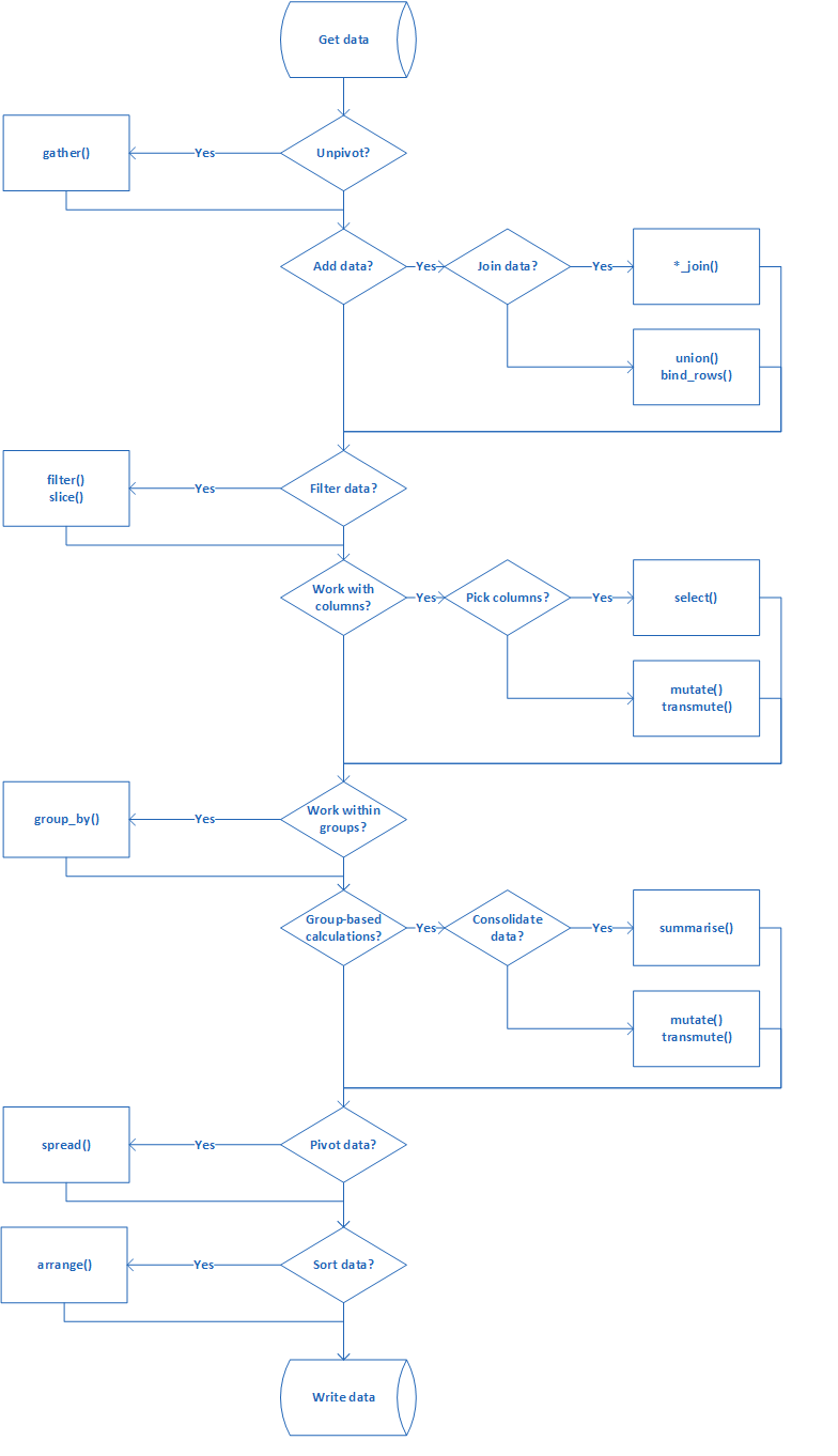
Putting it all together
This chapter gives a schematic diagram that details the steps to be performed
for any data munging exercise using tidyverse framework.
flights data
How many flights arrived late each month?
 1
 2
 3
 4
 5
 6
 7
 8
 9
10
11
12
13
14
15
16
17
18
19
| flights%>%
filter(arr_delay>5) %>%
group_by(month)%>%
summarise(n())
## # A tibble: 12 x 2
## month `n()`
## * <int> <int>
## 1 1 8988
## 2 2 8119
## 3 3 9033
## 4 4 10544
## 5 5 8490
## 6 6 10739
## 7 7 11518
## 8 8 9649
## 9 9 5347
## 10 10 7628
## 11 11 7485
## 12 12 12291
|
What percentage of traffic did each carrier represent, by month?
 1
 2
 3
 4
 5
 6
 7
 8
 9
10
11
12
13
14
15
16
17
18
19
20
21
22
23
24
25
| flights%>%
group_by(month, carrier)%>%
summarise(total=n()) %>%
ungroup()%>%
group_by(month)%>%
mutate(stotal = sum(total), pct = 100*total/stotal)%>%
ungroup()%>%
select(month,carrier, pct)%>%
spread(carrier,pct)
## # A tibble: 12 x 17
## month `9E` AA AS B6 DL EV F9 FL HA MQ OO
## <int> <dbl> <dbl> <dbl> <dbl> <dbl> <dbl> <dbl> <dbl> <dbl> <dbl> <dbl>
## 1 1 5.83 10.3 0.230 16.4 13.7 15.4 0.218 1.21 0.115 8.41 0.00370
## 2 2 5.85 10.1 0.224 16.4 13.8 15.3 0.196 1.19 0.112 8.19 NA
## 3 3 5.64 9.67 0.215 16.5 14.5 16.4 0.198 1.10 0.108 7.82 NA
## 4 4 5.33 9.61 0.212 15.9 14.4 16.1 0.201 1.10 0.106 7.80 NA
## 5 5 5.08 9.73 0.215 15.9 14.2 16.7 0.201 1.13 0.108 7.93 NA
## 6 6 5.09 9.76 0.212 16.4 14.6 15.8 0.195 0.892 0.106 7.71 0.00708
## 7 7 5.08 9.79 0.211 16.9 14.4 15.8 0.197 0.894 0.105 7.68 NA
## 8 8 4.96 9.74 0.211 16.9 14.7 15.6 0.188 0.897 0.106 7.72 0.0136
## 9 9 5.58 9.48 0.218 15.6 14.1 17.1 0.210 0.925 0.0907 8.00 0.0725
## 10 10 5.79 9.40 0.215 15.1 14.2 17.0 0.197 0.817 0.0727 7.71 NA
## 11 11 5.85 9.45 0.191 15.7 14.1 16.4 0.224 0.741 0.0917 7.54 0.0183
## 12 12 5.80 9.61 0.192 16.9 14.5 15.3 0.217 0.757 0.0995 7.60 NA
## # ... with 5 more variables: UA <dbl>, US <dbl>, VX <dbl>, WN <dbl>, YV <dbl>
|
What was the latest flight to depart each month?
 1
 2
 3
 4
 5
 6
 7
 8
 9
10
11
12
13
14
15
16
17
18
19
20
21
22
23
| flights%>%
group_by(month)%>%
arrange(desc(dep_time))%>%
slice_head(n=1)
## # A tibble: 12 x 19
## # Groups: month [12]
## year month day dep_time sched_dep_time dep_delay arr_time sched_arr_time
## <int> <int> <int> <int> <int> <dbl> <int> <int>
## 1 2013 1 7 2359 2359 0 506 437
## 2 2013 2 7 2400 2359 1 432 436
## 3 2013 3 15 2400 2359 1 324 338
## 4 2013 4 2 2400 2359 1 339 343
## 5 2013 5 21 2400 2359 1 339 350
## 6 2013 6 17 2400 2145 135 102 2315
## 7 2013 7 7 2400 1950 250 107 2130
## 8 2013 8 10 2400 2245 75 110 1
## 9 2013 9 2 2400 2359 1 411 340
## 10 2013 10 30 2400 2359 1 327 337
## 11 2013 11 27 2400 2359 1 515 445
## 12 2013 12 5 2400 2359 1 427 440
## # ... with 11 more variables: arr_delay <dbl>, carrier <chr>, flight <int>,
## # tailnum <chr>, origin <chr>, dest <chr>, air_time <dbl>, distance <dbl>,
## # hour <dbl>, minute <dbl>, time_hour <dttm>
|
gapminder data
Is there data for every key year for all countries?
1
2
3
| gapminder%>%group_by(year, country)%>%summarise(ct = n())%>%ungroup() %>%
spread(country,ct )%>%select(-year)%>%summarise_all(sum)%>%filter_all(all_vars(.!=12))%>%nrow()
## [1] 0
|
Provide an indexed GDP based on the earliest data###
 1
 2
 3
 4
 5
 6
 7
 8
 9
10
11
12
13
14
15
16
17
| index_vals <- gapminder %>% filter(year == min(year)) %>%
select(year, base=gdpPercap)
gapminder%>%inner_join(index_vals)%>%mutate(indexedgdp = gdpPercap/base)
## # A tibble: 20,164 x 8
## country continent year lifeExp pop gdpPercap base indexedgdp
## <fct> <fct> <int> <dbl> <int> <dbl> <dbl> <dbl>
## 1 Afghanistan Asia 1952 28.8 8425333 779. 779. 1
## 2 Afghanistan Asia 1952 28.8 8425333 779. 1601. 0.487
## 3 Afghanistan Asia 1952 28.8 8425333 779. 2449. 0.318
## 4 Afghanistan Asia 1952 28.8 8425333 779. 3521. 0.221
## 5 Afghanistan Asia 1952 28.8 8425333 779. 5911. 0.132
## 6 Afghanistan Asia 1952 28.8 8425333 779. 10040. 0.0776
## 7 Afghanistan Asia 1952 28.8 8425333 779. 6137. 0.127
## 8 Afghanistan Asia 1952 28.8 8425333 779. 9867. 0.0790
## 9 Afghanistan Asia 1952 28.8 8425333 779. 684. 1.14
## 10 Afghanistan Asia 1952 28.8 8425333 779. 8343. 0.0934
## # ... with 20,154 more rows
|
Takeaway
This book provides a very quick introduction to tidyverse framework. Along the
way, it highlight the main packages and functions that one tends to use in a
data munging exercise. It might be a useful read for anyone wanting a crash
course on tidyverse framework.