Faraway-2-Binomial Data
Purpose
To understand the way to model a linear relation if the Y variable is Binomial. There are lot of times when you encounter dependent variable being a Binomial.
The data being discusses is this : First column is the temperature at the time of launch Second column is the # of rings that got damaged.
> library(faraway) > data(orings) > orings$dam.prop <- orings$damage/6 > orings temp damage dam.prop 1 53 5 0.8333333 2 57 1 0.1666667 3 58 1 0.1666667 4 63 1 0.1666667 5 66 0 0.0000000 6 67 0 0.0000000 7 67 0 0.0000000 8 67 0 0.0000000 9 68 0 0.0000000 10 69 0 0.0000000 11 70 1 0.1666667 12 70 0 0.0000000 13 70 1 0.1666667 14 70 0 0.0000000 15 72 0 0.0000000 16 73 0 0.0000000 17 75 0 0.0000000 18 75 1 0.1666667 19 76 0 0.0000000 20 76 0 0.0000000 21 78 0 0.0000000 22 79 0 0.0000000 23 81 0 0.0000000 > par(mfrow = c(1, 1)) > plot(damage/6 ~ temp, orings, xlim = c(25, 85), ylim = c(0, 1), + xlab = "Temperature", ylab = "Prob of damage", pch = 19, + col = "blue") |
What would you do ?
> fit <- lm(dam.prop ~ temp, orings) > abline(fit) |
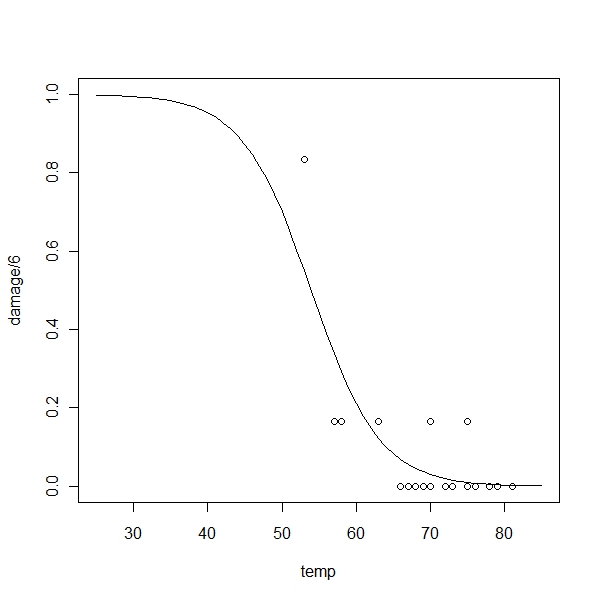
The above thing is obviously crap . So try fitting a logit model
> logitmod <- glm(cbind(damage, 6 - damage) ~ temp, family = binomial,
+     orings)
> summary(logitmod)
Call:
glm(formula = cbind(damage, 6 - damage) ~ temp, family = binomial,
    data = orings)

Deviance Residuals:
    Min       1Q   Median       3Q      Max
-0.9529  -0.7345  -0.4393  -0.2079   1.9565

Coefficients:
            Estimate Std. Error z value Pr(>|z|)
(Intercept) 11.66299    3.29626   3.538 0.000403 ***
temp        -0.21623    0.05318  -4.066 4.78e-05 ***
---
Signif. codes:  0 '***' 0.001 '**' 0.01 '*' 0.05 '.' 0.1 ' ' 1

(Dispersion parameter for binomial family taken to be 1)

    Null deviance: 38.898  on 22  degrees of freedom
Residual deviance: 16.912  on 21  degrees of freedom
AIC: 33.675

Number of Fisher Scoring iterations: 6
> plot(damage/6 ~ temp, orings, xlim = c(25, 85), ylim = c(0, 1))
> x <- seq(25, 85, 1)
> lines(x, ilogit(11.663 - 0.21628 * x)) |
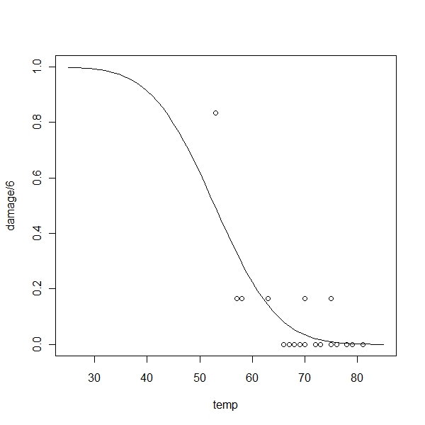
Now lets fit a probit
> probitmod <- glm(cbind(damage, 6 - damage) ~ temp, family = binomial(link = probit),
+     orings)
> summary(probitmod)
Call:
glm(formula = cbind(damage, 6 - damage) ~ temp, family = binomial(link = probit),
    data = orings)

Deviance Residuals:
    Min       1Q   Median       3Q      Max
-1.0134  -0.7760  -0.4467  -0.1581   1.9982

Coefficients:
            Estimate Std. Error z value Pr(>|z|)
(Intercept)  5.59145    1.71055   3.269  0.00108 **
temp        -0.10580    0.02656  -3.984 6.79e-05 ***
---
Signif. codes:  0 '***' 0.001 '**' 0.01 '*' 0.05 '.' 0.1 ' ' 1

(Dispersion parameter for binomial family taken to be 1)

    Null deviance: 38.898  on 22  degrees of freedom
Residual deviance: 18.131  on 21  degrees of freedom
AIC: 34.893

Number of Fisher Scoring iterations: 6
> plot(damage/6 ~ temp, orings, xlim = c(25, 85), ylim = c(0, 1))
> x <- seq(25, 85, 1)
> lines(x, pnorm(5.59145 - 0.1058 * x)) |
Residual deviance is the deviance of the current model when the null deviance is the deviance for a model with no predictors and just an intercept term Best way to test the model is as follows
> dev <- summary(probitmod)$null.deviance - summary(probitmod)$deviance > pchisq(dev, 1, lower = F) [1] 5.186666e-06 |
Thus you can see that the pvalue is so small the effect of temp is stat significant
Lets work on a probit model
> data(babyfood)
> head(babyfood)
  disease nondisease  sex   food
1      77        381  Boy Bottle
2      19        128  Boy  Suppl
3      47        447  Boy Breast
4      48        336 Girl Bottle
5      16        111 Girl  Suppl
6      31        433 Girl Breast
> babyfood$odds = babyfood$disease/babyfood$nondisease
> xtabs(disease/(disease + nondisease) ~ sex + food, babyfood)
      food
sex        Bottle     Breast      Suppl
  Boy  0.16812227 0.09514170 0.12925170
  Girl 0.12500000 0.06681034 0.12598425
> mdl <- glm(cbind(disease, nondisease) ~ sex + food, family = binomial,
+     babyfood)
> summary(mdl)
Call:
glm(formula = cbind(disease, nondisease) ~ sex + food, family = binomial,
    data = babyfood)

Deviance Residuals:
      1        2        3        4        5        6
 0.1096  -0.5052   0.1922  -0.1342   0.5896  -0.2284

Coefficients:
            Estimate Std. Error z value Pr(>|z|)
(Intercept)  -1.6127     0.1124 -14.347  < 2e-16 ***
sexGirl      -0.3126     0.1410  -2.216   0.0267 *
foodBreast   -0.6693     0.1530  -4.374 1.22e-05 ***
foodSuppl    -0.1725     0.2056  -0.839   0.4013
---
Signif. codes:  0 '***' 0.001 '**' 0.01 '*' 0.05 '.' 0.1 ' ' 1

(Dispersion parameter for binomial family taken to be 1)

    Null deviance: 26.37529  on 5  degrees of freedom
Residual deviance:  0.72192  on 2  degrees of freedom
AIC: 40.24

Number of Fisher Scoring iterations: 4
> drop1(mdl, test = "Chi")
Single term deletions

Model:
cbind(disease, nondisease) ~ sex + food
       Df Deviance    AIC    LRT   Pr(Chi)
<none>       0.722 40.240
sex     1    5.699 43.217  4.977   0.02569 *
food    2   20.899 56.417 20.177 4.155e-05 ***
---
Signif. codes: 0 '***' 0.001 '**' 0.01 '*' 0.05 '.' 0.1 ' ' 1 |
The choice of link function is crucial
> data(bliss) > bliss dead alive conc 1 2 28 0 2 8 22 1 3 15 15 2 4 23 7 3 5 27 3 4 > modl <- glm(cbind(dead, alive) ~ conc, family = binomial, data = bliss) > modp <- glm(cbind(dead, alive) ~ conc, family = binomial(link = probit), + data = bliss) > modc <- glm(cbind(dead, alive) ~ conc, family = binomial(link = cloglog), + data = bliss) > x <- seq(-2, 8, 0.2) > pl <- ilogit(modl$coef[1] + modl$coef[2] * x) > pp <- pnorm(modp$coef[1] + modp$coef[2] * x) > pc <- 1 - exp(-exp((modc$coef[1] + modc$coef[2] * x))) > par(mfrow = c(1, 3)) > plot(x, pl, type = "l", ylab = "Probability", xlab = "Dose") > lines(x, pp, lty = 2) > lines(x, pc, lty = 5) > matplot(x, cbind(pp/pl, (1 - pp)/(1 - pl)), type = "l", xlab = "Dose", + ylab = "Ratio") > matplot(x, cbind(pc/pl, (1 - pc)/(1 - pl)), type = "l", xlab = "Dose", + ylab = "Ratio") > par(mfrow = c(1, 1)) |
When does estimation fail ? I am tired of this chapter now as the data is increasingly non financial I have to cull out a dataset to make it interesting!!!