Hobson GLM - Chapter 7-1
Purpose
To work out the examples from Chap 7 Hobson’s book on GLM
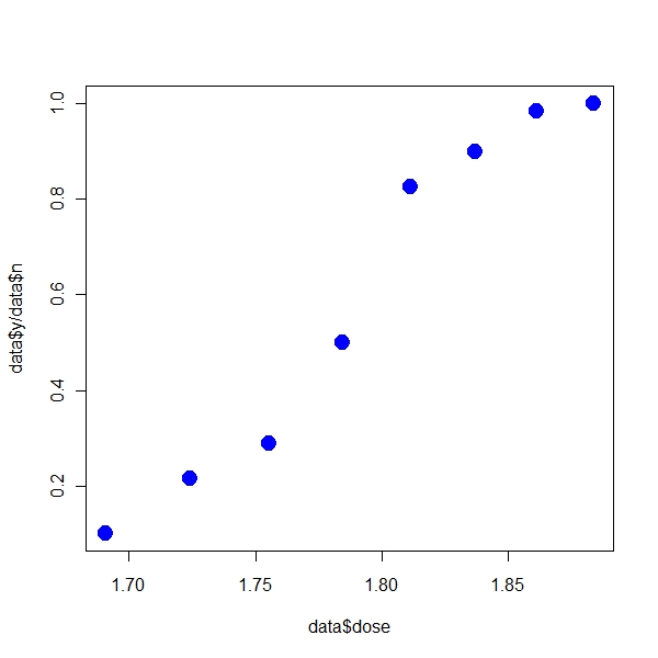
Beetle Mortality Example
> folder <- "C:/Cauldron/garage/R/soulcraft/Volatility/Learn/Dobson-GLM/" > file.input <- paste(folder, "Table 7.2 Beetle mortality.csv", + sep = "") > data <- read.csv(file.input, header = T, stringsAsFactors = F) > data$prop <- data$y/data$n > data$ny <- data$n - data$y |
> plot(data$dose, data$y/data$n, pch = 19, col = "blue", cex = 2) |
If I use R
> fit <- glm(formula = cbind(data$y, data$ny) ~ data$dose, family = binomial(link = "logit"))
> summary(fit)
Call:
glm(formula = cbind(data$y, data$ny) ~ data$dose, family = binomial(link = "logit"))

Deviance Residuals:
    Min       1Q   Median       3Q      Max
-1.5941  -0.3944   0.8329   1.2592   1.5940

Coefficients:
            Estimate Std. Error z value Pr(>|z|)
(Intercept)  -60.717      5.181  -11.72   <2e-16 ***
data$dose     34.270      2.912   11.77   <2e-16 ***
---
Signif. codes:  0 '***' 0.001 '**' 0.01 '*' 0.05 '.' 0.1 ' ' 1

(Dispersion parameter for binomial family taken to be 1)

    Null deviance: 284.202  on 7  degrees of freedom
Residual deviance:  11.232  on 6  degrees of freedom
AIC: 41.43

Number of Fisher Scoring iterations: 4 |
Example 1
Here’s the data .Coding up the likelihood function for poisson
> loglikf <- function(beta, data) {
+     t1 <- sum(data$y * (beta[1] + beta[2] * data$dose))
+     t2 <- sum(data$n * log(1 + exp(beta[1] + beta[2] * data$dose)))
+     t3 <- sum(log(choose(data$n, data$y)))
+     loglik <- t1 - t2 + t3
+     return(loglik)
+ } |
Using optim
> b1 <- 0.3 > b2 <- 0.3 > beta <- c(b1, b2) > solution <- optim(par = beta, fn = loglikf, control = list(fnscale = -2), + data = data) > print(solution$par) [1] -60.71904 34.27133 |
As you can see that both solutions are the same.