Purpose
To work on exercises from Dobson’s Book.
- Hiroshima Exercise
> folder <- "C:/Cauldron/garage/R/soulcraft/Volatility/Learn/Dobson-GLM/"
> file.input <- paste(folder, "Table 7.11 Hiroshima deaths.csv",
+ sep = "")
> data <- read.csv(file.input, header = T, stringsAsFactors = F)
> data <- data[1:6, ]
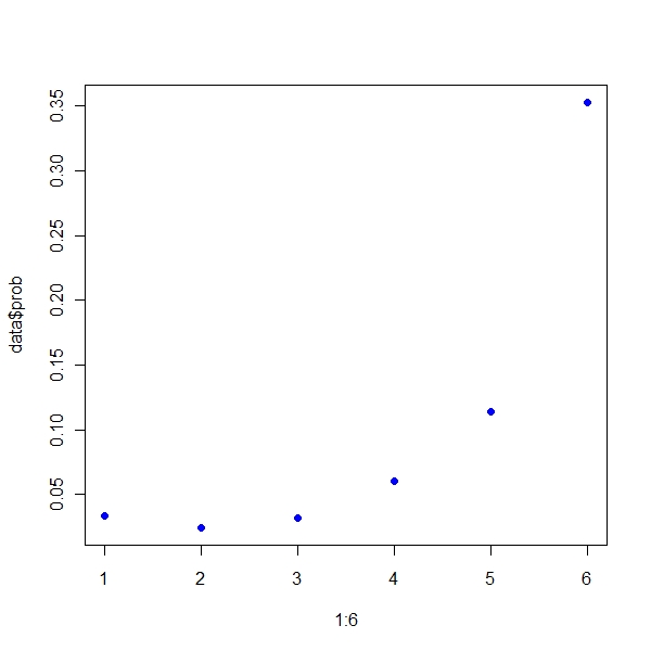
> data$prob <- data[, 2]/(data[, 2] + data[, 3])
> data$radiation <- factor(data$radiation) |
> plot(1:6, data$prob, pch = 19, col = "blue") |
Plot Log odds
> plot(1:6, log(data$prob/(1 - data$prob)), pch = 19, col = "blue") |
- Ok I took a peak at the solution and author uses lower bound of interval
> data$dose <- c(0, 1, 10, 50, 100, 200) |
- Use Logit
> fit <- glm(cbind(data$leukemia, data$other.cancer) ~ data$dose,
+     family = binomial(link = "logit"))
> summary(fit)
Call:
glm(formula = cbind(data$leukemia, data$other.cancer) ~ data$dose,
    family = binomial(link = "logit"))

Deviance Residuals:
         1           2           3           4           5           6
 0.4142808  -0.4899417  -0.1399059   0.0283528   0.0004824   0.0026940

Coefficients:
             Estimate Std. Error z value Pr(>|z|)
(Intercept) -3.488973   0.204062 -17.098  < 2e-16 ***
data$dose    0.014410   0.001817   7.932 2.15e-15 ***
---
Signif. codes:  0 '***' 0.001 '**' 0.01 '*' 0.05 '.' 0.1 ' ' 1

(Dispersion parameter for binomial family taken to be 1)

    Null deviance: 54.35089  on 5  degrees of freedom
Residual deviance:  0.43206  on 4  degrees of freedom
AIC: 26.097

Number of Fisher Scoring iterations: 4 |