NIFTY Returns Basic Number Crunching

Purpose : Look at NIFTY returns and Slice and dice to get a rough
idea of returns over many years

> library(xts)
> nifty <- read.csv("C:/Cauldron/Benchmark/Interns/nifty.csv",
+     header = T, stringsAsFactors = F)
> nifty$trade.date <- as.Date(nifty[, 1], format = "%d-%b-%y")
> nifty <- xts(nifty[, 2], nifty$trade.date)

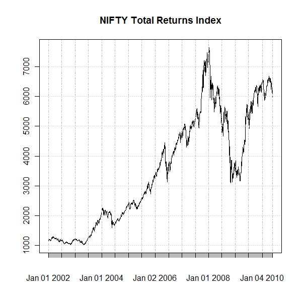
Plot Nifty Total Returns Indes

> plot(nifty, main = "NIFTY Total Returns Index")

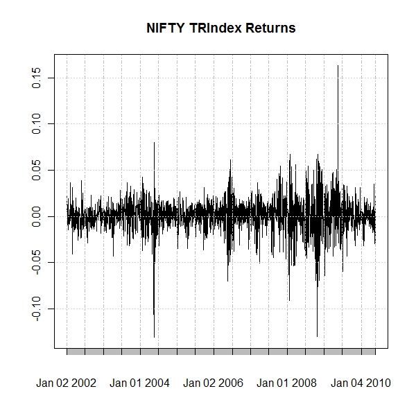
Plot NIFTY Total Ret Index - Daily returns

> nifty.ret <- as.xts(returns(nifty)[-1, ])
> plot(nifty.ret, main = "NIFTY TRIndex Returns", pch = 19, type = "l")

Prepare weekly, monthly, yearly, 2:10 yearly returns

> wid <- 5
> nifty.ret.weekly <- as.xts(rollapply(nifty.ret, width = wid,
+     sum, align = "right"))
> wid <- 20
> nifty.ret.monthly <- as.xts(rollapply(nifty.ret, width = wid,
+     sum, align = "right"))
> wid <- 125
> nifty.ret.sixmonthly <- as.xts(rollapply(nifty.ret, width = wid,
+     sum, align = "right"))
> wid <- 252
> nifty.ret.annual <- as.xts(rollapply(nifty.ret, width = wid,
+     sum, align = "right"))
> par(mfrow = c(2, 2))
> plot(nifty.ret.weekly, main = "Weekly Returns", pch = 19, type = "l")
> plot(nifty.ret.monthly, main = "Monthly Returns", pch = 19, type = "l")
> plot(nifty.ret.sixmonthly, main = "Six Monthly Returns", pch = 19,
+     type = "l")
> plot(nifty.ret.annual, main = "Annualized Returns", pch = 19,
+     type = "l")

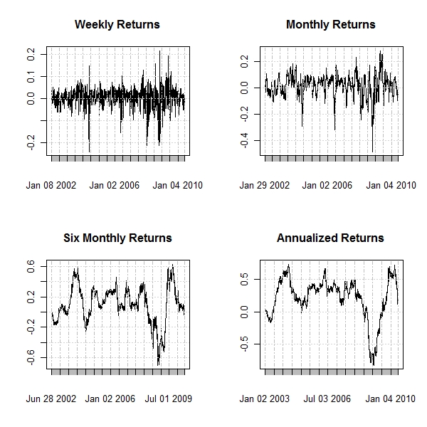
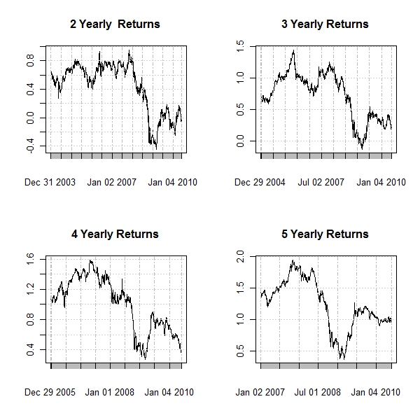
The more the holding period , the higher the frequency of obtaining higher returns

> wid <- 252 * 2
> nifty.ret.2yr <- as.xts(rollapply(nifty.ret, width = wid, sum,
+     align = "right"))
> wid <- 252 * 3
> nifty.ret.3yr <- as.xts(rollapply(nifty.ret, width = wid, sum,
+     align = "right"))
> wid <- 252 * 4
> nifty.ret.4yr <- as.xts(rollapply(nifty.ret, width = wid, sum,
+     align = "right"))
> wid <- 252 * 5
> nifty.ret.5yr <- as.xts(rollapply(nifty.ret, width = wid, sum,
+     align = "right"))
> par(mfrow = c(2, 2))
> plot(nifty.ret.2yr, main = "2 Yearly  Returns", pch = 19, type = "l")
> plot(nifty.ret.3yr, main = "3 Yearly Returns", pch = 19, type = "l")
> plot(nifty.ret.4yr, main = "4 Yearly Returns", pch = 19, type = "l")
> plot(nifty.ret.5yr, main = "5 Yearly Returns", pch = 19, type = "l")

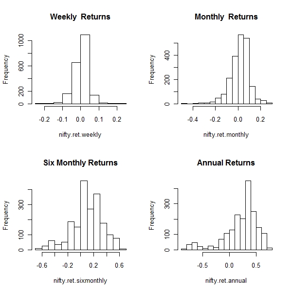
> par(mfrow = c(2, 2))
> hist(nifty.ret.weekly, main = "Weekly  Returns")
> hist(nifty.ret.monthly, main = "Monthly  Returns")
> hist(nifty.ret.sixmonthly, main = "Six Monthly Returns")
> hist(nifty.ret.annual, main = "Annual Returns")

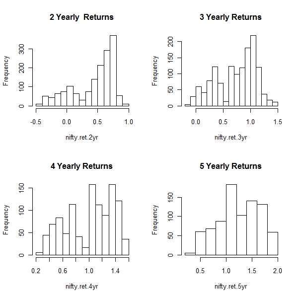
> par(mfrow = c(2, 2))
> hist(nifty.ret.2yr, main = "2 Yearly  Returns")
> hist(nifty.ret.3yr, main = "3 Yearly Returns")
> hist(nifty.ret.4yr, main = "4 Yearly Returns")
> hist(nifty.ret.5yr, main = "5 Yearly Returns")

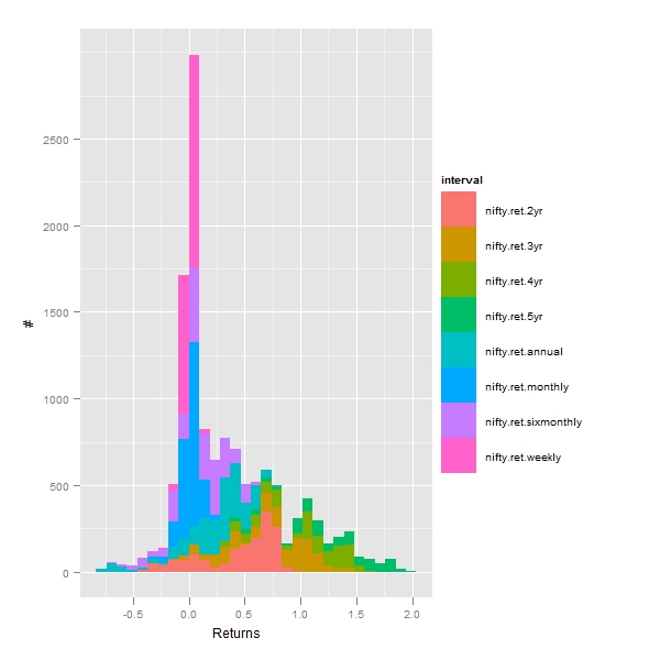
> library(ggplot2)
> z <- merge(nifty.ret.weekly, nifty.ret.monthly, nifty.ret.sixmonthly,
+     nifty.ret.annual, nifty.ret.2yr, nifty.ret.3yr, nifty.ret.4yr,
+     nifty.ret.5yr)
> z1 <- data.frame(coredata(z))
> z2 <- stack(z1)
> colnames(z2) <- c("returns", "interval")
> p <- ggplot(z2, aes(x = returns, fill = interval))
> q <- p + geom_histogram() + scale_x_continuous("Returns")
> q <- q + scale_y_continuous("#")
> print(q)

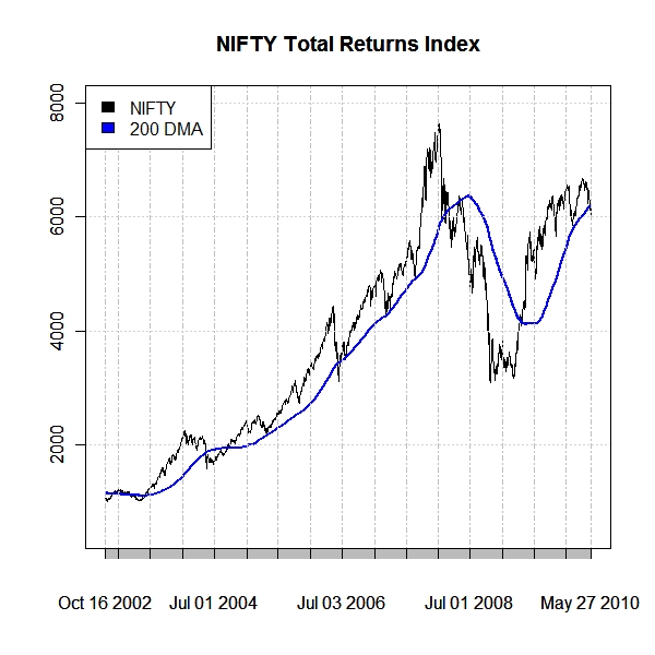
Comparison of 200 day Moving Average of NIFTY and NIFTY

> par(mfrow = c(1, 1))
> wid <- 200
> nifty.ma.200 <- as.xts(rollapply(nifty, width = wid, mean, align = "right"))
> temp <- merge(nifty, nifty.ma.200)
> temp <- temp[(!is.na(temp[, 2])), ]
> plot(temp[, 1], main = "NIFTY Total Returns Index", ylim = c(500,
+     8000))
> par(new = T)
> plot(temp[, 2], main = "NIFTY Total Returns Index", ylim = c(500,
+     8000), col = "blue", lwd = 2)
> legend("topleft", legend = c("NIFTY", "200 DMA"), fill = c("black",
+     "blue"))