Histogram Characteristics
Purpose
To deep practice histogram
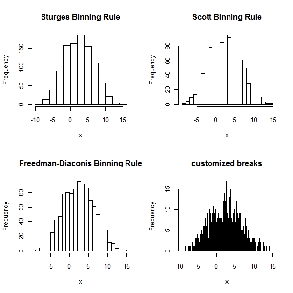
> x <- rnorm(1000, 2, 4) + runif(200) > par(mfrow = c(2, 2)) > hist(x, main = "Sturges Binning Rule") > hist(x, breaks = "Scott", main = "Scott Binning Rule") > hist(x, breaks = "Freedman-Diaconis", main = "Freedman-Diaconis Binning Rule") > hist(x, breaks = seq(min(x) - 1, max(x) + 1, 0.1), main = "customized breaks") |
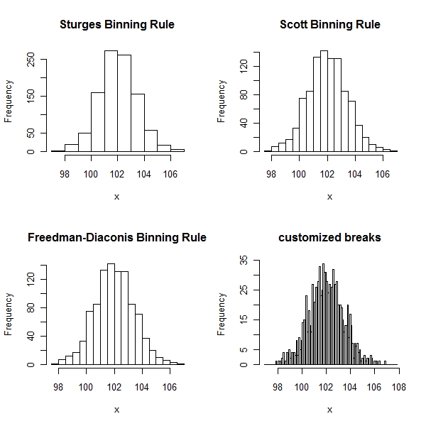
Histograms are useful only so much… If you mix two normals , then whatever method
you choose , you do not get the true picture out of a histogram
> x <- rnorm(1000, 2, 1) + rnorm(1000, 100, 1) > par(mfrow = c(2, 2)) > hist(x, main = "Sturges Binning Rule") > hist(x, breaks = "Scott", main = "Scott Binning Rule") > hist(x, breaks = "Freedman-Diaconis", main = "Freedman-Diaconis Binning Rule") > hist(x, breaks = seq(min(x) - 1, max(x) + 1, 0.1), main = "customized breaks") |
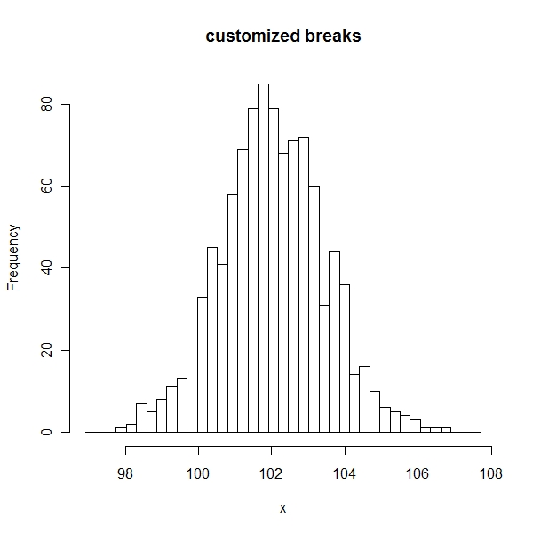
Using methods from smoothing methodology (Hardle, Muller, Sperlich and Werwatz, 2003) one can find an optimal binwidth h for n observations:
> par(mfrow = c(1, 1)) > h <- (24 * sqrt(pi)/2000)^(1/3) > hist(x, breaks = seq(min(x) - 1, max(x) + 1, h), main = "customized breaks") |