Chi Plot
Purpose
Use Chi Plot to study randomness
The funda behind the plot is to look at a non parametric estimator of joint distribution of the 2 variables and marginals. Subsequently create a plot with respect to lambda versus chi.
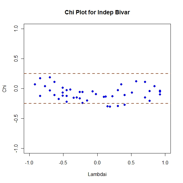
Independent Bivariates
> n <- 50 > x <- array(rnorm(50)) > y <- array(rnorm(50)) > z <- cbind(x, y) > Fi <- apply(x, 1, function(temp) length(which(x[which(x != temp)] <= + temp))/(n - 1)) > Gi <- apply(y, 1, function(temp) length(which(y[which(y != temp)] <= + temp))/(n - 1)) > Hi <- apply(z, 1, function(temp) length(which(x[which(x != temp[1])] <= + temp[1] & y[which(y != temp[2])] <= temp[2]))/(n - 1)) > Chi <- (Hi - Fi * Gi)/sqrt(Fi * (1 - Fi) * Gi * (1 - Gi)) > Lambdai <- 4 * sign((Fi - 0.5) * (Gi - 0.5)) * pmax((Fi - 0.5)^2, + (Gi - 0.5)^2) > result <- cbind(Lambdai, Chi) > condition <- abs(result[, 1]) < 4 * (1/(n - 1) - 0.5)^2 > not.consid <- n - sum(condition) > result <- (result[condition, ]) > cp <- 1.78 > par(mfrow = c(1, 1)) > plot(Lambdai, Chi, pch = 19, col = "blue", ylim = c(-1, 1), main = "Chi Plot for Indep Bivar") > abline(h = c(-1, 1) * cp/sqrt(n), col = "sienna", lwd = 2, lty = "dashed") |
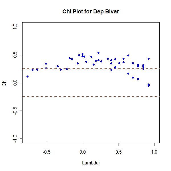
Dependent Bivariates
> library(mnormt) > n <- 50 > sample.mean <- c(0, 0) > sample.cov <- matrix(c(1, 0.7, 0.7, 1), nrow = 2) > z <- rmnorm(n, mean = sample.mean, varcov = sample.cov) > x <- array(z[, 1]) > y <- array(z[, 2]) > Fi <- apply(x, 1, function(temp) length(which(x[which(x != temp)] <= + temp))/(n - 1)) > Gi <- apply(y, 1, function(temp) length(which(y[which(y != temp)] <= + temp))/(n - 1)) > Hi <- apply(z, 1, function(temp) length(which(x[which(x != temp[1])] <= + temp[1] & y[which(y != temp[2])] <= temp[2]))/(n - 1)) > Chi <- (Hi - Fi * Gi)/sqrt(Fi * (1 - Fi) * Gi * (1 - Gi)) > Lambdai <- 4 * sign((Fi - 0.5) * (Gi - 0.5)) * pmax((Fi - 0.5)^2, + (Gi - 0.5)^2) > result <- cbind(Lambdai, Chi) > condition <- abs(result[, 1]) < 4 * (1/(n - 1) - 0.5)^2 > not.consid <- n - sum(condition) > result <- (result[condition, ]) > cp <- 1.78 > par(mfrow = c(1, 1)) > plot(Lambdai, Chi, pch = 19, col = "blue", ylim = c(-1, 1), main = "Chi Plot for Dep Bivar") > abline(h = c(-1, 1) * cp/sqrt(n), col = "sienna", lwd = 2, lty = "dashed") |
Let me see whether chiplot code can be made in to a function or not
> n <- 50
> sample.mean <- c(0, 0)
> sample.cov <- matrix(c(1, 0.7, 0.7, 1), nrow = 2)
> z <- rmnorm(n, mean = sample.mean, varcov = sample.cov)
> GetChiPlotData <- function(z) {
+     n <- dim(z)[1]
+     x <- array(z[, 1])
+     y <- array(z[, 2])
+     Fi <- apply(x, 1, function(temp) length(which(x[which(x !=
+         temp)] <= temp))/(n - 1))
+     Gi <- apply(y, 1, function(temp) length(which(y[which(y !=
+         temp)] <= temp))/(n - 1))
+     Hi <- apply(z, 1, function(temp) length(which(x[which(x !=
+         temp[1])] <= temp[1] & y[which(y != temp[2])] <= temp[2]))/(n -
+         1))
+     Chi <- (Hi - Fi * Gi)/sqrt(Fi * (1 - Fi) * Gi * (1 - Gi))
+     Lambdai <- 4 * sign((Fi - 0.5) * (Gi - 0.5)) * pmax((Fi -
+         0.5)^2, (Gi - 0.5)^2)
+     result <- cbind(Lambdai, Chi)
+     condition <- abs(result[, 1]) < 4 * (1/(n - 1) - 0.5)^2
+     not.consid <- n - sum(condition)
+     result <- (result[condition, ])
+     return(list(result = result, not.considered = not.consid))
+ }
> print(GetChiPlotData(z))
$result
          Lambdai       Chi
 [1,]  0.57017909 0.3817040
 [2,] -0.77009579 0.2211629
 [3,]  0.40024990 0.3426714
 [4,]  0.77009579 0.3185426
 [5,]  0.84339858 0.3151982
 [6,] -0.63348605 0.1819625
 [7,]  0.15035402 0.6322076
 [8,]  0.70012495 0.5172935
 [9,]  0.63348605 0.4423879
[10,]  0.84339858 0.4787234
[11,]  0.18367347 0.4647580
[12,]  0.05039567 0.6446564
[13,]  0.35027072 0.3800585
[14,] -0.03373594 0.6475506
[15,] -0.22032486 0.5204165
[16,]  0.57017909 0.1964671
[17,]  0.40024990 0.5026842
[18,]  0.63348605 0.2233177
[19,]  0.35027072 0.4544504
[20,]  0.30362349 0.3271425
[21,]  0.51020408 0.1538968
[22,]  0.18367347 0.3302891
[23,]  0.57017909 0.1985712
[24,] -0.07038734 0.5176139
[25,]  0.22032486 0.4798488
[26,] -0.01041233 0.6023524
[27,] -0.12036651 0.5150819
[28,]  0.40024990 0.3567158
[29,]  0.30362349 0.1987769
[30,] -0.26030820 0.5579887
[31,]  0.51020408 0.2830693
[32,]  0.26030820 0.4455119
[33,]  0.77009579 0.1461864
[34,]  0.45356102 0.4024390
[35,]  0.84339858 0.2962532
[36,] -0.18367347 0.5252257
[37,] -0.45356102 0.3987333
[38,]  0.70012495 0.4714045
[39,]  0.51020408 0.4508348
[40,] -0.15035402 0.4624973
[41,]  0.57017909 0.4693807
[42,]  0.35027072 0.4557193
[43,]  0.35027072 0.3228829
[44,]  0.26030820 0.1831267

$not.considered
[1] 6 |
I will use this function from now on to see the dependency structure