Understanding Tail Dependencies using Chi-Plot

Purpose
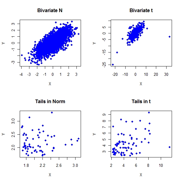
Use Chi plots to look at 1. Tail Dependencies ? 2. Are tail dependencies symmetric or asymmetric ? 3. Spot Outliers

Prepare Data

> library(mnormt)
> n <- 3000
> sample.mean <- c(0, 0)
> sample.cov <- matrix(c(1, 0.7, 0.7, 1), nrow = 2)
> z1 <- rmnorm(n, mean = sample.mean, varcov = sample.cov)
> z2 <- rmt(n, mean = sample.mean, S = sample.cov, df = 3)
> z1.x <- quantile(z1[, 1], prob = seq(0, 1, 0.05))[20]
> z1.y <- quantile(z1[, 2], prob = seq(0, 1, 0.05))[20]
> condition1 <- (z1[, 1] > z1.x) & (z1[, 2] > z1.y)
> z2.x <- quantile(z2[, 1], prob = seq(0, 1, 0.05))[20]
> z2.y <- quantile(z2[, 2], prob = seq(0, 1, 0.05))[20]
> condition2 <- (z2[, 1] > z2.x) & (z2[, 2] > z2.y)
> par(mfrow = c(2, 2))
> plot(z1, col = "blue", pch = 19, main = "Bivariate N", xlab = "X",
+     ylab = "Y")
> plot(z2, col = "blue", pch = 19, main = "Bivariate t", xlab = "X",
+     ylab = "Y")
> plot(z1[condition1, ], col = "blue", pch = 19, main = "Tails in Norm",
+     xlab = "X", ylab = "Y")
> plot(z2[condition2, ], col = "blue", pch = 19, main = "Tails in t",
+     xlab = "X", ylab = "Y")

ChiPlots

> GetChiPlotData <- function(z) {
+     n <- dim(z)[1]
+     x <- array(z[, 1])
+     y <- array(z[, 2])
+     Fi <- apply(x, 1, function(temp) length(which(x[which(x !=
+         temp)] <= temp))/(n - 1))
+     Gi <- apply(y, 1, function(temp) length(which(y[which(y !=
+         temp)] <= temp))/(n - 1))
+     Hi <- apply(z, 1, function(temp) length(which(x[which(x !=
+         temp[1])] <= temp[1] & y[which(y != temp[2])] <= temp[2]))/(n -
+         1))
+     Chi <- (Hi - Fi * Gi)/sqrt(Fi * (1 - Fi) * Gi * (1 - Gi))
+     Lambdai <- 4 * sign((Fi - 0.5) * (Gi - 0.5)) * pmax((Fi -
+         0.5)^2, (Gi - 0.5)^2)
+     result <- cbind(Lambdai, Chi)
+     return(result)
+ }
> cp <- 1.78
> z1c <- GetChiPlotData(z1)
> z2c <- GetChiPlotData(z2)
> master1 <- cbind(z1, z1c)
> master2 <- cbind(z2, z2c)

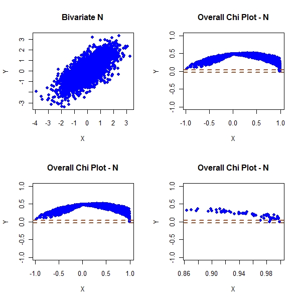
> par(mfrow = c(2, 2))
> plot(master1[, 1], master1[, 2], col = "blue", pch = 19, main = "Bivariate N",
+     xlab = "X", ylab = "Y")
> plot(master1[, 3], master1[, 4], pch = 19, col = "blue", ylim = c(-1,
+     1), main = "Overall Chi Plot - N", xlab = "X", ylab = "Y")
> abline(h = c(-1, 1) * cp/sqrt(n), col = "sienna", lwd = 2, lty = "dashed")
> plot(master1[!condition1, 3], master1[!condition1, 4], pch = 19,
+     col = "blue", ylim = c(-1, 1), main = "Overall Chi Plot - N",
+     xlab = "X", ylab = "Y")
> abline(h = c(-1, 1) * cp/sqrt(n), col = "sienna", lwd = 2, lty = "dashed")
> plot(master1[condition1, 3], master1[condition1, 4], pch = 19,
+     col = "blue", ylim = c(-1, 1), main = "Overall Chi Plot - N",
+     xlab = "X", ylab = "Y")
> abline(h = c(-1, 1) * cp/sqrt(n), col = "sienna", lwd = 2, lty = "dashed")

> par(mfrow = c(2, 2))
> plot(master2[, 1], master2[, 2], col = "blue", pch = 19, main = "Bivariate N",
+     xlab = "X", ylab = "Y")
> plot(master2[, 3], master2[, 4], pch = 19, col = "blue", ylim = c(-1,
+     1), main = "Overall Chi Plot - N", xlab = "X", ylab = "Y")
> abline(h = c(-1, 1) * cp/sqrt(n), col = "sienna", lwd = 2, lty = "dashed")
> plot(master2[!condition2, 3], master2[!condition2, 4], pch = 19,
+     col = "blue", ylim = c(-1, 1), main = "Overall Chi Plot - N",
+     xlab = "X", ylab = "Y")
> abline(h = c(-1, 1) * cp/sqrt(n), col = "sienna", lwd = 2, lty = "dashed")
> plot(master2[condition2, 3], master2[condition2, 4], pch = 19,
+     col = "blue", ylim = c(-1, 1), main = "Overall Chi Plot - N",
+     xlab = "X", ylab = "Y")
> abline(h = c(-1, 1) * cp/sqrt(n), col = "sienna", lwd = 2, lty = "dashed")

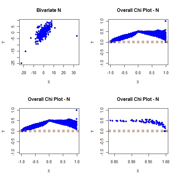
Look at the above plots. You can clearly see the tail dependence
The t joint dist shows that the tail dependence no longer goes to 0. This is unlike gaus joint which shows that tail dependence goes to 0.

A marvelous way to visualize tail dependencies.