MDS
Purpose
Exploratory Multivariate Analysis from Venables and Ripley
This is basic Factor analysis plot
> data(iris3)
> ir <- rbind(iris3[, , 1], iris3[, , 2], iris3[, , 3])
> ir.species <- factor(c(rep("s", 50), rep("c", 50), rep("v", 50)))
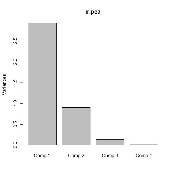
> ir.pca <- princomp(log(ir), cor = T)
> summary(ir.pca)
Importance of components:
Comp.1 Comp.2 Comp.3 Comp.4
Standard deviation 1.7124583 0.9523797 0.36470294 0.1656840
Proportion of Variance 0.7331284 0.2267568 0.03325206 0.0068628
Cumulative Proportion 0.7331284 0.9598851 0.99313720 1.0000000
> plot(ir.pca)
> loadings(ir.pca)
Loadings:
Comp.1 Comp.2 Comp.3 Comp.4
Sepal L. 0.504 -0.455 0.709 0.191
Sepal W. -0.302 -0.889 -0.331
Petal L. 0.577 -0.219 -0.786
Petal W. 0.567 -0.583 0.580
Comp.1 Comp.2 Comp.3 Comp.4
SS loadings 1.00 1.00 1.00 1.00
Proportion Var 0.25 0.25 0.25 0.25
Cumulative Var 0.25 0.50 0.75 1.00 |
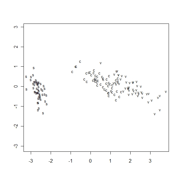
MDS
> ir.scal <- cmdscale(dist(ir), k = 2, eig = T) > ir.scal$points[, 2] <- -ir.scal$points[, 2] > eqscplot(ir.scal$points, type = "n") > text(ir.scal$points, labels = as.character(ir.species), cex = 0.8) > distp <- dist(ir) > dist2 <- dist(ir.scal$points) > sum((distp - dist2)^2/sum(distp^2)) [1] 0.001746943 |
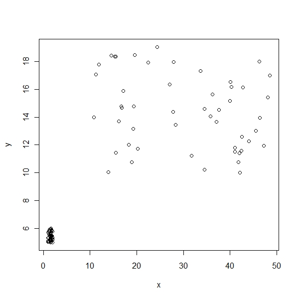
Let me simulate a dataset with 2 dimensions
> x <- cbind(runif(50, 10, 50), runif(50, 1, 2))
> y <- cbind(runif(50, 10, 20), runif(50, 5, 6))
> z <- rbind(x, y)
> lab <- c(rep("A", 50), rep("B", 50))
> plot(x, y) |
> ir.scal <- cmdscale(dist(z), k = 2, eig = T) > ir.scal$points[, 2] <- -ir.scal$points[, 2] > eqscplot(ir.scal$points, type = "n") > text(ir.scal$points, labels = as.character(lab), cex = 0.8) |
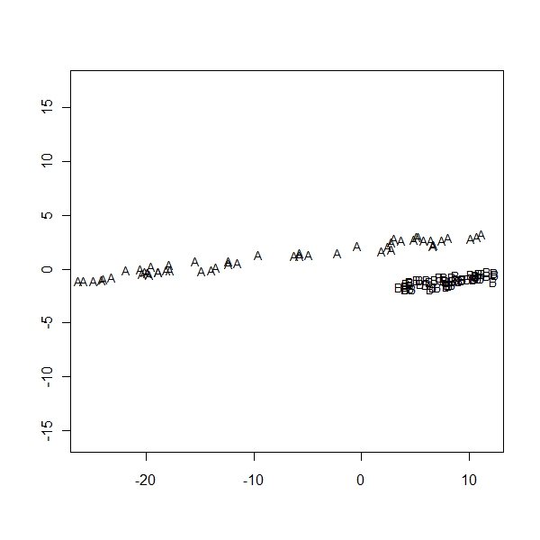
I get a basic idea of Multidimensional Scaling… But the actual math behind it is not really clear!!! Got to read Kruskal and Wish Monograph to get a more detailed understanding of the math behind it..