Legendre Polynomials
Purpose
Discrete Legendre Polynomials Build a Vandermonde Matrix
> library(RColorBrewer)
> x <- (-128:128)/128
> A <- cbind(x^0, x, x^2, x^3)
> Q <- qr.Q(qr(A))
> par(mfrow = c(1, 1))
> cols <- brewer.pal(4, "Set1")
> plot(x, Q[, 1], ylim = c(-0.2, 0.2), col = cols[1], ylab = "",
+     pch = 19)
> par(new = T)
> plot(x, Q[, 2], ylim = c(-0.2, 0.2), col = cols[2], ylab = "",
+     pch = 19)
> par(new = T)
> plot(x, Q[, 3], ylim = c(-0.2, 0.2), col = cols[3], ylab = "",
+     pch = 19)
> par(new = T)
> plot(x, Q[, 4], ylim = c(-0.2, 0.2), col = cols[4], ylab = "",
+     pch = 19, main = "Legendre Polynomials")
> abline(h = 0, col = "grey", lty = "dashed")
> abline(v = 0, col = "grey", lty = "dashed")
> legend("topleft", legend = c("P0", "P1", "P2", "P3"), fill = cols) |
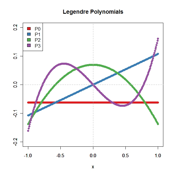
By starting with any basis ( 1, x , x^2, ..) we can generate an orthonormal basis by QR factorization. Once this is done, you can project any function in this orthogonal space and all the computations become a charm.
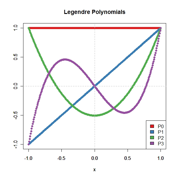
Scale the stuff
> D <- diag(1/Q[257, ])
> Q1 <- Q %*% D
> par(mfrow = c(1, 1))
> cols <- brewer.pal(4, "Set1")
> plot(x, Q1[, 1], ylim = c(-1, 1), col = cols[1], ylab = "", pch = 19)
> par(new = T)
> plot(x, Q1[, 2], ylim = c(-1, 1), col = cols[2], ylab = "", pch = 19)
> par(new = T)
> plot(x, Q1[, 3], ylim = c(-1, 1), col = cols[3], ylab = "", pch = 19)
> par(new = T)
> plot(x, Q1[, 4], ylim = c(-1, 1), col = cols[4], ylab = "", pch = 19,
+     main = "Legendre Polynomials")
> abline(h = 0, col = "grey", lty = "dashed")
> abline(v = 0, col = "grey", lty = "dashed")
> legend("bottomright", legend = c("P0", "P1", "P2", "P3"), fill = cols) |