Machine Epsilon
Purpose
To work out Experiment 2 from the numerical linear algebra
> set.seed(12345) > U <- qr.Q(qr(matrix(rnorm(6400), ncol = 80, nrow = 80))) > V <- qr.Q(qr(matrix(rnorm(6400), ncol = 80, nrow = 80))) > S <- diag(2^(-1:-80)) > A <- U %*% S %*% V |
Classic Gram-Schmidt function
> classic.gs <- function(A) {
+     m <- dim(A)[1]
+     n <- dim(A)[2]
+     Q <- matrix(data = NA, nrow = m, ncol = n)
+     Q[, 1] <- A[, 1]
+     Q[, 1] <- Q[, 1]/sqrt(sum(Q[, 1]^2))
+     j <- 2
+     for (j in 2:n) {
+         vj <- A[, j]
+         for (i in 1:(j - 1)) {
+             rij <- t(Q[, i]) * A[, j]
+             vj <- vj - rij * Q[, i]
+         }
+         rjj <- sqrt(sum(vj^2))
+         qj <- vj/rjj
+         Q[, j] <- qj
+     }
+     return(Q)
+ } |
> Q.classic <- classic.gs(A) > R.classic <- solve(Q.classic, A) > Q <- qr.Q(qr(A)) > R <- qr.R(qr(A)) > rii.classic <- diag(R.classic) > rii.mod <- diag(R) |
> library(RColorBrewer) > cols <- brewer.pal(4, "Set1") > par(mfrow = c(1, 2)) > plot(1:80, abs(rii.classic), log = "y", ylab = "", , col = cols[1], + pch = 19) > plot(1:80, abs(rii.mod), log = "y", ylab = "", , col = cols[2], + pch = 19) |
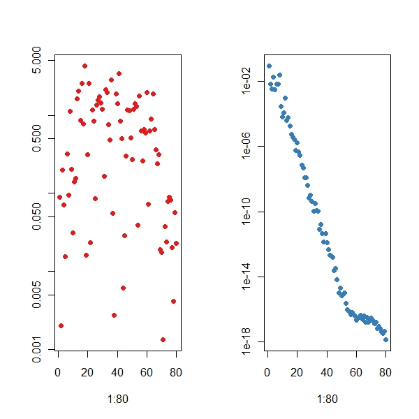
The above example is a superb one which shows the level of machine epsilon. WOW! Life is so beautiful when you live at depths