Difference between Polynomial and Expansion
Purpose
Floating point arithmetic explained in Trefethen_Bau
> library(polynom)
> p <- polynomial(1)
> for (i in 1:9) {
+     p <- p * polynomial(c(-2, 1))
+ }
> print(p)
-512 + 2304*x - 4608*x^2 + 5376*x^3 - 4032*x^4 + 2016*x^5 - 672*x^6 + 144*x^7 -
18*x^8 + x^9
> q <- as.function(p) |
> t <- seq(-1.92, 2.08, by = 0.001) > library(RColorBrewer) > cols <- brewer.pal(4, "Set1") > par(mfrow = c(1, 2)) > yran <- range(q(t)) > plot(t, q(t), ylim = yran, pch = 19, col = cols[1]) > plot(t, (t - 2)^9, ylim = yran, pch = 19, col = cols[2]) |
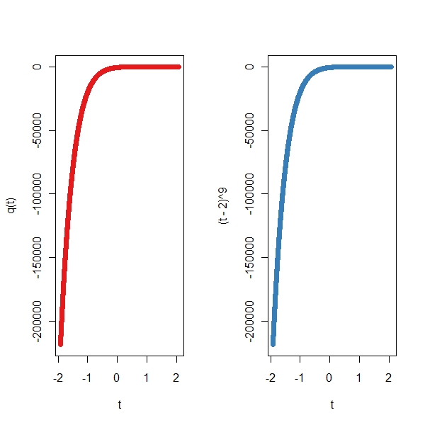
Lets plot the difference
> par(mfrow = c(1, 1)) > plot(t, q(t) - (t - 2)^9, pch = 19, col = cols[3]) |
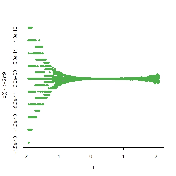
One can see that very near to x = -2 , there is a difference of 10^-10 between the two expressions. But at positive x = 2, there is hardly any difference.