Fitting Distribution in R
Purpose
Is to work through FITTING DISTRIBUTIONS WITH R Release 0.4-21 February 2005 It is a 6 year old document but I think I should get my hands dirty a bit to be a plug and play mode.Also , any revisit of this document will make me think in a different way.
There are four steps in fitting distributions 1. Model/funtion choice 2. Estimate parameters 3. Evaluate goodness of fit 4. Goodness of fit statistical tests
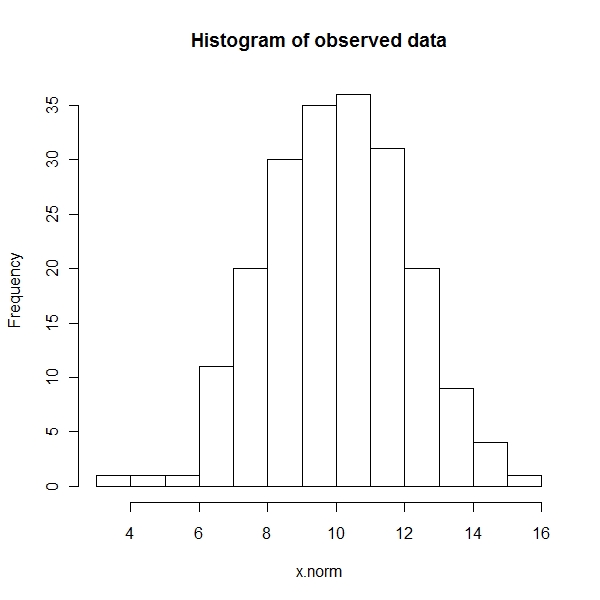
Histogram
> x.norm <- rnorm(n = 200, m = 10, sd = 2) > hist(x.norm, main = "Histogram of observed data") |
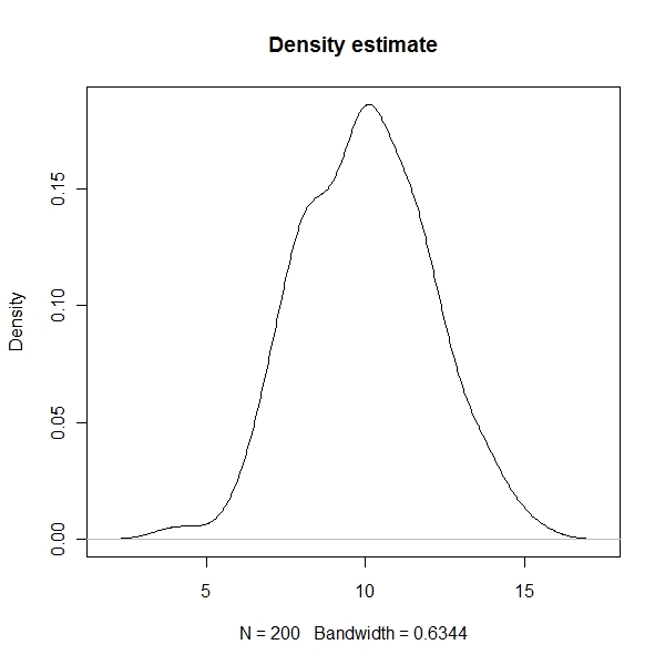
Density state
> plot(density(x.norm), main = "Density estimate") |
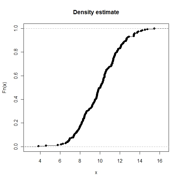
ECDF state
> plot(ecdf(x.norm), main = "Density estimate") |
This is something I learnt today
qqplot can be used to check any sample distribution with theoretical distribution
> x.wei <- rweibull(n = 200, shape = 2.1, scale = 1.1) > x.teo <- rweibull(n = 200, shape = 2, scale = 1) > qqplot(x.teo, x.wei, main = "QQ-plot distr. Weibull") > abline(0, 1) |
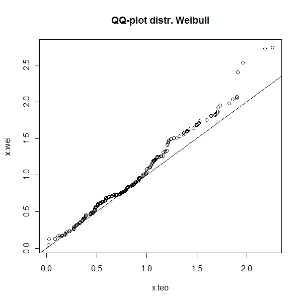
The biggest challenge is that , curves only differ by mean, variability, skewness and kurtosis. So, if you standardize the variables, the a functional form with both skewness and kurtosis can be used to check the distribution
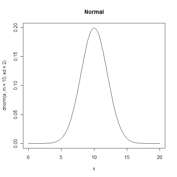
Normal
> curve(dnorm(x, m = 10, sd = 2), from = 0, to = 20, main = "Normal") |
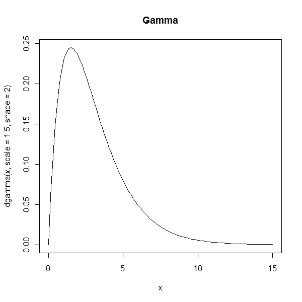
Gamma
> curve(dgamma(x, scale = 1.5, shape = 2), from = 0, to = 15, main = "Gamma") |
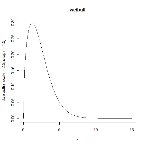
Weibull
> curve(dweibull(x, scale = 2.5, shape = 1.5), from = 0, to = 15, + main = "weibull") |
Skewness and Kurtosis for Normal Distribution
> library(fBasics) > skewness(x.norm) [1] 0.0132836 attr(,"method") [1] "moment" > kurtosis(x.norm) [1] -0.1502271 attr(,"method") [1] "excess" |
Skewness and Kurtosis for Weibull
> skewness(x.wei) [1] 0.8799243 attr(,"method") [1] "moment" > kurtosis(x.wei) [1] 0.5694369 attr(,"method") [1] "excess" |
Check normal
> x <- rnorm(1000, 2, 3)
> fitdistr(x, "normal")
      mean          sd
  2.02103915   3.06295954
(0.09685929) (0.06848986) |
Check gamma
> x <- rgamma(1000, 2, 3)
> fitdistr(x, "gamma")
     shape         rate
  2.11176055   3.22441614
(0.08800314) (0.15158757) |
Check pois
> x <- rpois(1000, 2)
> fitdistr(x, "poisson")
     lambda
  1.96500000
(0.04432832) |
Look at the amazing collection that this fitdistr can be used to check the distributions
Chi-Square goodness of fit
> n <- 200
> x.pois <- rpois(n, 2.5)
> lambda.est <- mean(x.pois)
> tab.os <- table(x.pois)
> freq.os <- vector()
> for (i in 1:length(tab.os)) {
+     freq.os[i] <- tab.os[[i]]
+ }
> freq.ex <- dpois((0:max(x.pois)), lambda = lambda.est) * n
> acc <- mean(abs(freq.os - trunc(freq.ex)))
> acc * 100/mean(freq.os)
[1] 16.5 |
I began going through this 24 page document to check whether a particular distribution comes from cauchy.
Let me generate a gaussian normal variable and check whether it comes from cauchy
> x <- rnorm(1000, 0, 1)
> h <- hist(x, breaks = 20)
> y <- rcauchy(1000, 0)
> y.cut <- cut(y, breaks = h$breaks)
> observed.freq <- as.vector(table(y.cut))/1000
> expected.freq <- as.vector(h$density)
> temp <- 0
> for (i in seq_along(observed.freq)) {
+     temp <- temp + ((observed.freq[i] - expected.freq[i])^2)/expected.freq[i]
+ }
> dof <- length(observed.freq) - 2 - 1
> pchisq(temp, dof)
[1] 1 |
This p is extremely small and hence one can reject the null hypothesis.
Obviously sample from cauchy is vastly different from sample from normal
Another learning is the package vcd which can be used to check goodness of fit
> library(vcd)
> y <- rpois(1000, 2)
> gf <- goodfit(y, type = "poisson", method = "MinChisq")
> summary(gf)
         Goodness-of-fit test for poisson distribution

             X^2 df  P(> X^2)
Pearson 5.228552 7 0.6320941 |