First Brush with Lattice

Purpose
To explore grid package

> library(grid)
> library(lattice)

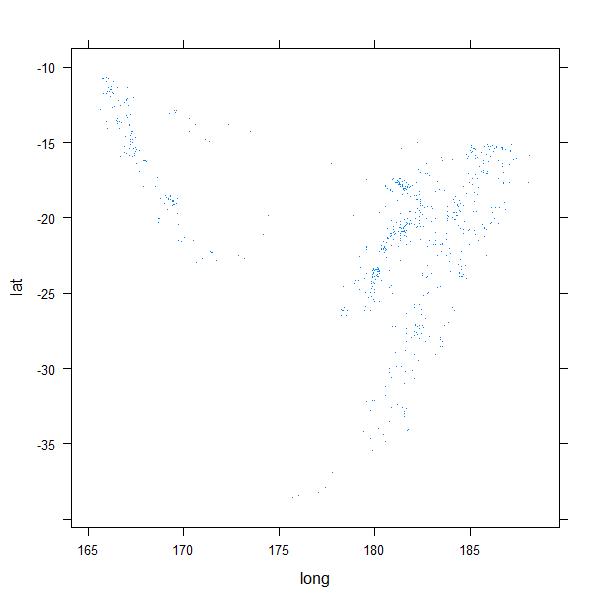
Basic xyplot

> xyplot(lat ~ long, data = quakes, pch = ".")

Store the plot in a tplot

> tplot <- xyplot(lat ~ long, data = quakes, pch = ".")
> print(tplot)

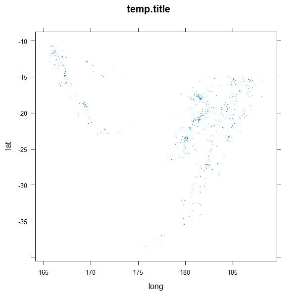
Update the tplot produced

> tplot <- xyplot(lat ~ long, data = quakes, pch = ".")
> print(update(tplot, main = "temp.title"))

> x <- 1:5
> y <- 1:5
> g <- factor(1:5)
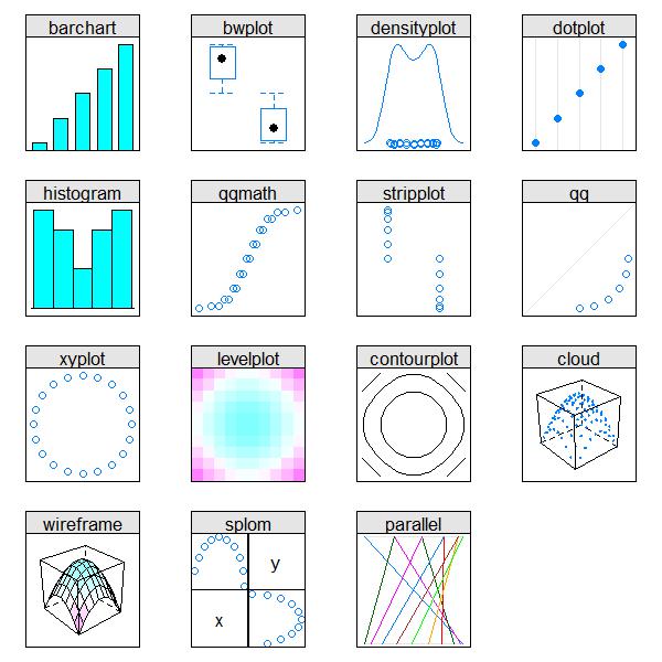
> types <- c("barchart", "bwplot", "densityplot", "dotplot", "histogram",
+     "qqmath", "stripplot", "qq", "xyplot", "levelplot", "contourplot",
+     "cloud", "wireframe", "splom", "parallel")
> angle <- seq(0, 2 * pi, length = 21)[-21]
> xx <- cos(angle)
> yy <- sin(angle)
> gg <- factor(rep(1:2, each = 10))
> aaa <- seq(0, pi, length = 10)
> xxx <- rep(aaa, 10)
> yyy <- rep(aaa, each = 10)
> zzz <- sin(xxx) + sin(yyy)
> doplot <- function(name, ...) {
+     do.call(name, list(..., scales = list(draw = FALSE), xlab = NULL,
+         ylab = NULL, strip = function(which.panel, ...) {
+             grid.rect(gp = gpar(fill = "grey90"))
+             grid.text(name)
+         }))
+ }
> plot <- vector("list", 15)
> plot[[1]] <- doplot("barchart", y ~ g | 1)
> plot[[2]] <- doplot("bwplot", yy ~ gg | 1, par.settings = list(box.umbrella = list(lwd = 0.5)))
> plot[[3]] <- doplot("densityplot", ~yy | 1)
> plot[[4]] <- doplot("dotplot", y ~ g | 1)
> plot[[5]] <- doplot("histogram", ~yy | 1)
> plot[[6]] <- doplot("qqmath", ~yy | 1)
> plot[[7]] <- doplot("stripplot", yy ~ gg | 1)
> plot[[8]] <- doplot("qq", gg ~ yy | 1)
> plot[[9]] <- doplot("xyplot", xx ~ yy | 1)
> plot[[10]] <- doplot("levelplot", zzz ~ xxx + yyy | 1, colorkey = FALSE)
> plot[[11]] <- doplot("contourplot", zzz ~ xxx + yyy | 1, labels = FALSE,
+     cuts = 8)
> plot[[12]] <- doplot("cloud", zzz ~ xxx + yyy | 1, zlab = NULL,
+     zoom = 0.9, par.settings = list(box.3d = list(lwd = 0.01)))
> plot[[13]] <- doplot("wireframe", zzz ~ xxx + yyy | 1, zlab = NULL,
+     zoom = 0.9, drape = TRUE, par.settings = list(box.3d = list(lwd = 0.01)),
+     colorkey = FALSE)
> plot[[14]] <- doplot("splom", ~data.frame(x = xx[1:10], y = yy[1:10]) |
+     1, pscales = 0)
> plot[[15]] <- doplot("parallel", ~data.frame(x = xx[1:10], y = yy[1:10]) |
+     1)
> grid.newpage()
> pushViewport(viewport(layout = grid.layout(4, 4)))
> for (i in 1:15) {
+     pushViewport(viewport(layout.pos.col = ((i - 1)%%4) + 1,
+         layout.pos.row = ((i - 1)%/%4) + 1))
+     print(plot[[i]], newpage = FALSE, panel.width = list(1.025,
+         "inches"), panel.height = list(1.025, "inches"))
+     popViewport()
+ }
> popViewport()

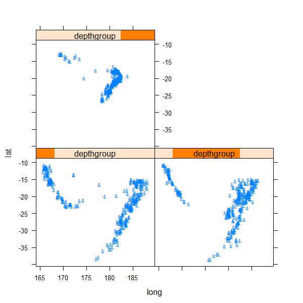
Shingle - The first term that needs to be understood in the context of lattice

> depthgroup <- equal.count(quakes$depth, number = 3, overlap = 0)
> p <- (xyplot(lat ~ long | depthgroup, data = quakes, pch = "&"))
> print(p)

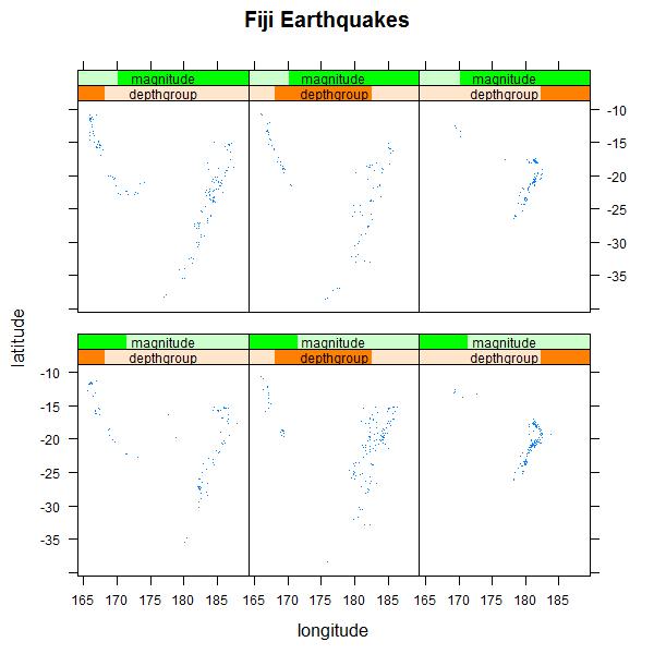
A non trivial example of using lattice to produce conditioned plots

> magnitude <- equal.count(quakes$mag, number = 2, overlap = 0)
> p <- xyplot(lat ~ long | depthgroup * magnitude, data = quakes,
+     main = "Fiji Earthquakes", ylab = "latitude", xlab = "longitude",
+     pch = ".", scales = list(x = list(alternating = c(1, 1, 1))),
+     between = list(y = 1), par.strip.text = list(cex = 0.7),
+     par.settings = list(axis.text = list(cex = 0.7)))
> print(p)

To get the default settings

> trellis.par.get("fontsize")
$text
[1] 12

$points
[1] 8

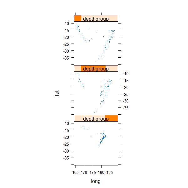
To customize the layout of the graphic

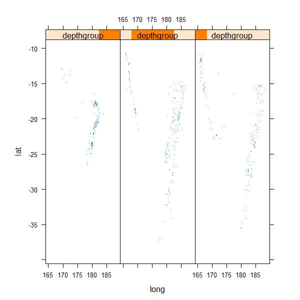
> depthgroup <- equal.count(quakes$depth, number = 3, overlap = 0)
> p <- xyplot(lat ~ long | depthgroup, data = quakes, pch = ".",
+     layout = c(1, 3), aspect = 1, index.cond = list(3:1))
> print(p)

aspect can be used to control the height of the panel.

> depthgroup <- equal.count(quakes$depth, number = 3, overlap = 0)
> p <- xyplot(lat ~ long | depthgroup, data = quakes, pch = ".",
+     layout = c(3, 1), aspect = 1, index.cond = list(3:1))
> print(p)

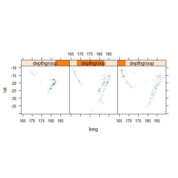
aspect can be used to control the height of the panel.

> depthgroup <- equal.count(quakes$depth, number = 3, overlap = 0)
> p <- xyplot(lat ~ long | depthgroup, data = quakes, pch = ".",
+     layout = c(3, 1), aspect = 2, index.cond = list(3:1))
> print(p)

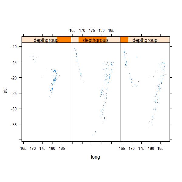
aspect can be used to control the height of the panel.

> depthgroup <- equal.count(quakes$depth, number = 3, overlap = 0)
> p <- xyplot(lat ~ long | depthgroup, data = quakes, pch = ".",
+     layout = c(3, 1), aspect = 3, index.cond = list(3:1))
> print(p)

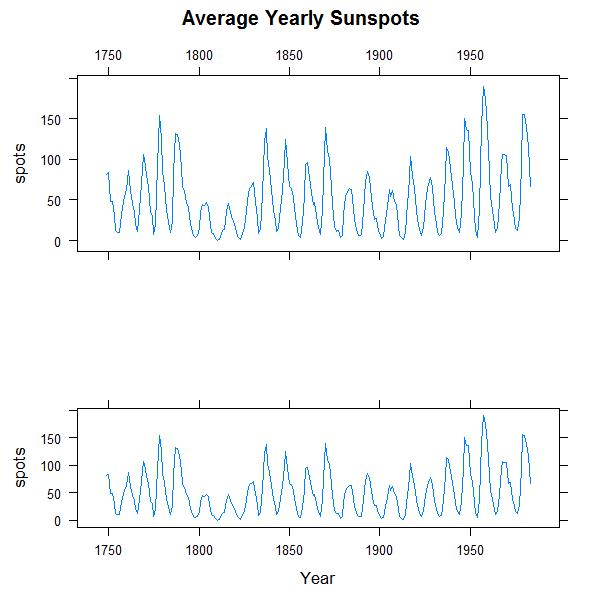
Showing various lattice plots in a customized way

> spots <- by(sunspots, gl(235, 12, lab = 1749:1983), mean)
> plot1 <- xyplot(spots ~ 1749:1983, xlab = "", type = "l", main = "Average Yearly Sunspots",
+     scales = list(x = list(alternating = 2)))
> plot2 <- xyplot(spots ~ 1749:1983, xlab = "Year", type = "l")
> print(plot1, position = c(0, 0.2, 1, 1), more = TRUE)
> print(plot2, position = c(0, 0, 1, 0.33))

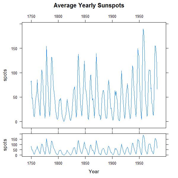
Position : A vector of 4 numbers, typically c(xmin, ymin, xmax, ymax) that give the lower-left and upper-right corners of a rectangle in which the Trellis plot of x is to be positioned. The coordinate system for this rectangle is [0-1] in both the x and y directions.

Experimenting with the positions

> spots <- by(sunspots, gl(235, 12, lab = 1749:1983), mean)
> plot1 <- xyplot(spots ~ 1749:1983, xlab = "", type = "l", main = "Average Yearly Sunspots",
+     scales = list(x = list(alternating = 2)))
> plot2 <- xyplot(spots ~ 1749:1983, xlab = "Year", type = "l")
> print(plot1, position = c(0.005, 0.5, 1, 1), more = TRUE)
> print(plot2, position = c(0.005, 0, 1, 0.4))