Cracked density() function
After 3 weeks and close to 2 days of constant thinking about density functions, I have finally cracked the density function in base R.My head was spinning in all directions and I could not get my hands on cracking it.
Finally I did what any failed person would do to learn something. Start from scratch
Firstly I wrote my own R code to do kernel density estimation
> gauss.wt <- function(x) {
+     1/(sqrt(2 * pi)) * exp(-x^2/2)
+ }
> set.seed(1977)
> n <- 512
> obs.c <- sample(c(1, 2), n, T)
> mus <- c(3, 7)
> sigs <- c(1, 1)
> x <- sapply(obs.c, function(x) rnorm(1, mus[x], sigs[x]))
> n <- length(x)
> h <- bw.nrd0(x)
> prob <- sapply(x, function(z) (1/(n * h)) * sum(gauss.wt((z -
+     x)/h)))
> z <- cbind(x, prob)
> z <- z[order(x), ] |
> par(mfrow = c(1, 1)) > plot(prob ~ x, type = "l", data = z, xlim = range(x), ylim = c(0, + 0.2), col = "red", lwd = 3) |
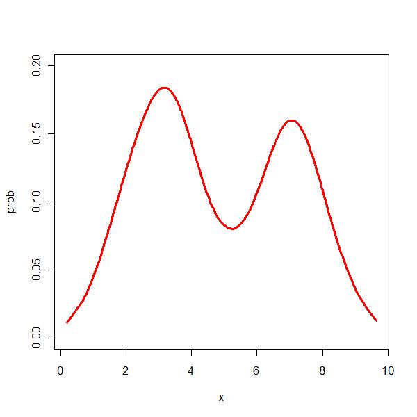
Ok, it looks like KDE
Now I wanted to compare with base R output
> res <- density(x) > prob1 <- approx(res$x, res$y, z[, 1]) |
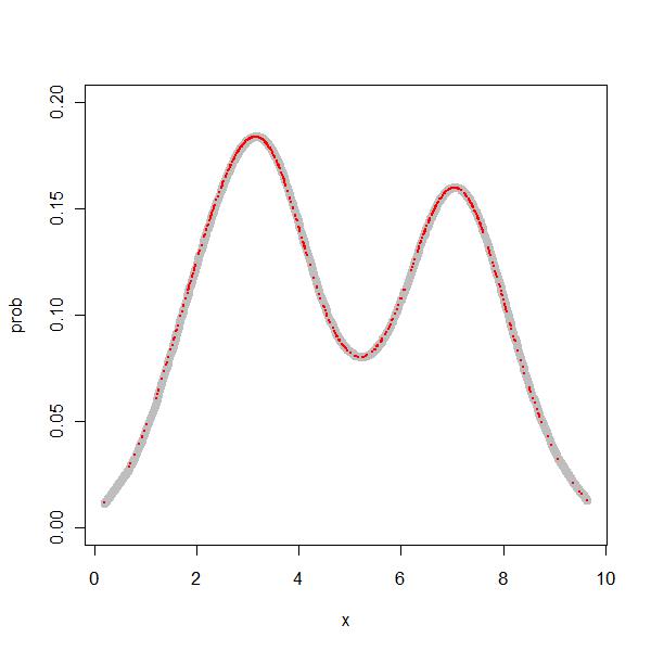
So, I was able to get the density values at all the relevant points.
> par(mfrow = c(1, 1)) > plot(prob ~ x, type = "l", data = z, xlim = range(x), ylim = c(0, + 0.2), col = "grey", lwd = 8) > points(z[, 1], prob1$y, col = "red", lty = "dashed", cex = 0.2, + pch = 19) |

This was the first mini achievement. I could manually replicate the density function
Now the next task was to customize density function of R and code my own. I download the R source code, read through the C file that was being used in the density function and replicated the C code in R.
> density.rad <- function(x, bw = "nrd0", n = 512, cut = 3) {
+     x <- as.vector(x)
+     weights <- rep.int(1/n, n)
+     n <- max(n, 512)
+     if (n > 512)
+         n <- 2^ceiling(log2(n))
+     bw <- bw.nrd0(x)
+     from <- min(x) - cut * bw
+     to <- max(x) + cut * bw
+     lo <- from - 4 * bw
+     up <- to + 4 * bw
+     BinDist <- function(x, weights, lo, up, n) {
+         y <- numeric(2 * n)
+         xdelta <- (up - lo)/n
+         for (i in seq_along(x)) {
+             xpos <- (x[i] - lo)/xdelta
+             ix <- floor(xpos)
+             fx <- xpos - ix
+             wi <- weights[i]
+             y[ix] <- y[ix] + (1 - fx) * wi
+             y[ix + 1] <- y[ix + 1] + (fx) * wi
+         }
+         return(y)
+     }
+     y <- BinDist(x, weights, lo, up, n)
+     kords <- seq.int(0, 2 * (up - lo), length.out = 2L * n)
+     kords[(n + 2):(2 * n)] <- -kords[n:2]
+     kords <- dnorm(kords, sd = bw)
+     kords <- fft(fft(y) * Conj(fft(kords)), inverse = TRUE)
+     kords <- pmax.int(0, Re(kords)[1L:n]/length(y))
+     xords <- seq.int(lo, up, length.out = n)
+     x <- seq.int(from, to, length.out = n)
+     list(x = x, y = approx(xords, kords, x)$y)
+ } |
> res <- density.rad(x) > prob1 <- approx(res$x, res$y, z[, 1]) |
So, I was able to get the density values at all the relevant points.
> par(mfrow = c(1, 1)) > plot(prob ~ x, type = "l", data = z, xlim = range(x), ylim = c(0, + 0.2), col = "grey", lwd = 8) > points(z[, 1], prob1$y, col = "red", lty = "dashed", cex = 0.2, + pch = 19) |
So, finally I have achieved a mini milestone, i.e. understanding the density function at a certain depth.
I am still unclear on the convolution front. Let me take some time and understand that aspect. But for now , let me blog this. After a very long time , I feel that I have cracked something nice. I had been going through a lot of troubles to understand this.