Robust Portfolio Optimization & Management : Summary

I tend to read books from the Fabozzi factory ![]() , not to get mathematical rigor in a subject but to get an intuitive understanding of the stuff. Overtime, this approach has helped me managed my expectations from Fabozzi books. Having never worked on Black-Litterman model till date, I wanted to get some intuition behind the model. With that mindset, I went through the book. The book is divided into four parts**. Part I** covers classical portfolio theory and its modern extensions. **Part II** introduces traditional and modern frameworks for robust estimation of returns. **Part III** provides readers with the necessary background for handling the optimization part of portfolio management. **Part IV** focuses on applications of the robust estimation and optimization methods described in the previous parts, and outlines recent trends and new directions in robust portfolio management and in the investment management industry in general. The structure of the book is pretty logical. Starting off with the basic principles of modern portfolio management, one moves on to understanding estimation process, and then understanding the optimization process and finally exploring new directions.
, not to get mathematical rigor in a subject but to get an intuitive understanding of the stuff. Overtime, this approach has helped me managed my expectations from Fabozzi books. Having never worked on Black-Litterman model till date, I wanted to get some intuition behind the model. With that mindset, I went through the book. The book is divided into four parts**. Part I** covers classical portfolio theory and its modern extensions. **Part II** introduces traditional and modern frameworks for robust estimation of returns. **Part III** provides readers with the necessary background for handling the optimization part of portfolio management. **Part IV** focuses on applications of the robust estimation and optimization methods described in the previous parts, and outlines recent trends and new directions in robust portfolio management and in the investment management industry in general. The structure of the book is pretty logical. Starting off with the basic principles of modern portfolio management, one moves on to understanding estimation process, and then understanding the optimization process and finally exploring new directions.
PART I - Portfolio Allocation : Classic Theory and Extensions
Mean Variance Analysis and Modern Portfolio Theory
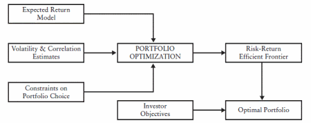
Investment process as seen from Modern Portfolio management

Mean variance framework refers to a specific problem formulation wherein one tries to minimize risk for a specific level of return OR maximize return for a specific level of risk. The objective function usually is set as a quadratic programming problem where the constraints are formulated for asset weights. These constraints typically specify the target risk and the bounds on asset weights. If there is no target return constraint specified, the resulting portfolio is called the global minimum variance portfolio. Obviously there is a limit to the diversification benefits that an investor can seek. Just by adding limitless number of assets, the portfolio risk does not vanish. Instead it approaches a constant
Minimizing variance for a target mean is just one type of formulating fund manager’s problem. There can be other variants, depending on the fund manager’s context and fund objective. Some of the alternative formulations are explored in this chapter such as expected return maximization formulation, Risk aversion formulation, etc.
The efficient set of portfolios available to investors who employ mean-variance analysis in the absence of risk-free asset is inferior to that available when there is a risk-free asset. When one includes a risk-free asset, the asset allocation is reduced to a line, called “Capital Market Line”. The portfolios on this line are nothing but some combination of risk-free asset and minimum variance portfolios. The point at which the line hits the frontier is called “tangency portfolio”, also called the market portfolio. Hence all the portfolios on the CML line represent combination of borrowing or lending at the risk-free rate and investing in the market portfolio. This property is called the “separation”.
Utility functions are then introduced to measure the investor’s preferences for a portfolio with a certain risk and return characteristics.
If we choose the quadratic utility function, then the utility function maximization coincides with mean variance framework.
Advances in the theory of Portfolio Risk measures
If investor’s decision making process is dependent beyond the first moments, one needs to modify or work with an alternative framework than the mean variance framework. There are two types of risk measures explored in this chapter, Dispersion measures & Downside measures. Dispersion measures are measures of uncertainty. In contrast to downside measures, dispersion measures consider both positive and negative deviations from the mean, and treat those deviations as equally risky. Some common portfolio dispersion approaches are mean standard deviation, mean-variance, mean-absolute deviation, and mean-absolute moment. Some common portfolio downside measures are Roy’s safety-first, semi variance, lower partial moment, Value-at-Risk, and Conditional Value-at-Risk. In all these methods, some variant of utility maximization procedure is employed.
Portfolio Selection in Practice
There are usually constraints imposed on the mean variance framework. This chapter gives a basic classification of the constraints, which are
- Linear and Quadratic constraints
- Long-Only constraints
- Turnover constraints
- Holding constraints
- Risk factor constraints
- Benchmark Exposure and Tracking error constraints
- General Linear and Quadratic constraints
- Combinatorial and Integer constraints
- Minimum-Holding and Transaction size constraints
- Cardinality constraints
- Round lot constraints
Portfolio optimization problems with minimum holding constraints, cardinality constraints or round lot constraints are so-called NP-complete. For the practical solution of these problems heuristics and approximation techniques are used.
In practice, few portfolio managers go to the extent of including constraints of this type in their optimization framework. Instead, a standard mean-variance optimization problem is solved and then, in a “post-optimization” step, generated portfolio weights or trades are pruned to satisfy the constraints. This simplification leads to small, but often negligible, differences compared to a full optimization using the threshold constraints. The chapter then gives a flavor of incorporating transaction costs in asset allocation models. A simple and straightforward approach is to assume a separable transaction cost function that is dependent only on the weights of the assets in the portfolio. An alternate approach is to assume a piece-wise linear dependence between the assets and trade size. As such the models might appear complex, but this area is well explored in the finance literature. Piece-wise linear approximations for transactions cost are solver friendly. There is an enormous breadth of material that is covered in this book and it sometimes is overwhelming. For example the case of multi-account optimization does sound very complex to understand in the first reading.
PART II – Robust Parameter Estimation.
Classical Asset Pricing
This chapter gives a crash course on simple random walks, arithmetic random walks, geometric random walks, trend stationary processes, covariance stationary processes, etc. that one sees in the finance literature.
Forecasting Expected Risk and Return
The basic problem with mean variance framework is that one uses historical data estimates of mean return and covariance to use it in the asset allocation decisions for the future. There is a forecast that is built in to plain vanilla mean variance framework. Ideally an estimate should have the following characteristics
· It provides a forward-looking forecast with some predictive power, not just backward looking historical summary of past performance
-
The estimate can be produced at a reasonable cost
-
The technique does not amplify errors already present in the inputs used in the process of intuition
-
The forecast should be intuitive, i.e, portfolio manager or the analyst should be able to explain and justify them in a comprehensible manner.
It is typically observed that sample mean and sample covariance have a low forecasting power. It is obvious as the asset returns are typically the realization of a stochastic process and in fact could a complete random walk as some believe it to be and vehemently argue for the same.
The chapter goes on to introduce basic dividend discount models, which I think are basically pointless and dumbest way to do formulate estimates. Using sample mean and covariance is also fraught with danger. Sample mean is a good predictor only for distributions that are not heavy-tailed. However most of the financial time series are heavy tailed and non-stationary and hence the resulting estimator has a large estimation error. In my own little exercise that I have done using some assets in the Indian markets, I found that
-
Equally weight portfolios offer a comparable advantage to using asset allocation using sample mean and sample covariance
-
Uncertainty of mean completely plays a spoil sport in efficient asset allocation. It is sometimes ok to have an estimation error in covariance, but estimation error in mean kills the performance of asset allocation
-
Mean variance portfolios are not diversified properly. In fact one can calculate zephyr drift score for the portfolios and one can easily see that there is a considerable variance in the portfolio composition.
What are the possible remedies that one can use?
For expected returns, one can use a factor model / Black-Litterman model / Shrinkage estimators. Remedies can easily be talked about, but the implementation is difficult. Black-Litterman needs views about assets, views about the error estimates of the views. So, you take these subjective views and then try to build a model based on Bayesian statistics. In the real world for a small boutique shop offering asset allocation solutions, who provides these views? How to put weights on these opinions? I really wonder the reason behind this immense popularity of Black-Litterman model. Can it really outperform a naïve portfolio? My current frame of mind suggests it might not beat a naïve 1/N portfolio.
For Covariance matrix, there are remedies too, but the effectiveness is context specific and sometimes completely questionable. Sample covariance matrix is essentially a non-parametric estimator. One can put a structure for the covariance matrix and then estimate it. Jagannathan and Ma suggest using portfolios of covariance matrix estimators. Shrinkage estimator is another way to work on it. The crucial thing to ponder upon is ,” If the estimator is a better estimate , does it actually give a higher out-of sample Sharpe ratio ? “.The chapter then talks about Heteroskedasticity and Autocorrelation consistent covariance matrix estimation. It talks about the treatment for covariance matrix under varying lengths, increasing the sampling frequency etc. Overall this gives the reader a broad sense of estimators that can be used for covariance matrix. Chow’s method is mentioned where the covariance matrix is built using the two covariance matrices ,one in quieter period and another in noisy period. Well, how to combine these matrices could be as simple as relying on intuition , or complex way by considering a markov chain. Another remedy suggested is in using a different volatility metric , i.e one of the downside measures such as semi-variance etc. .
Random matrices are introduced to show the importance of dimensionality reduction. It can be shown in cases where the asset universe is large, there are a few eigen values which dominate the rest. Hence random matrix theory makes a case for using factor based model like APT. Again factor models can themselves be of multiple varieties. They can be statistical factor models, macroeconomic factor models, fundamental factor models etc. Selecting the “optimal number of factors” is a dicey thing. The selection criteria should be in such a way that it reduces estimation error and bias. Too less factors decreases estimation error but increases bias. Too many factors increase estimator error but decrease bias. So, I guess the ideal number of factors and type of factors to choose is more an art than science. One of the strong reasons for using a factor model is the obvious dimensional reduction for a large asset universe allocation problem.
The chapter also mentions various methods for estimating volatility such as modeling it based on the implied vols of the relevant options,use clustering techniques, use GARCH methods or use stochastic vol methods. One must remember though that most of these methods are relevant in the Q world (sell side) and not the P world( buy side).
Robust Estimation
Robust estimation is not just a fancy way of removing outliers and estimating parameters. It is a fundamentally different way of estimation. If one is serious about understanding it thoroughly, it is better to skip this chapter as the content merely does a lip service to the various concepts.
Robust Framework for Estimation: Shrinkage, Bayesian Approaches and Black-Litterman Model
Estimation of expected returns and covariance matrix is subjected to estimation error in practice. The portfolio weights change constantly and resulting in the considerable portfolio turnover and sub-optimal realization of portfolio returns. What can be done to remedy such a situation?
There can be two areas where one can improve things. On the estimation side, one can employ estimates that are less sensitive to outliers, estimators such as shrinkage estimators, Bayesian estimators. On the modeling side, one can constrain portfolio weights, use portfolio resampling, or apply robust or stochastic optimization techniques to specify scenarios or ranges of values for parameters estimated from data, thus incorporating uncertainty in to the optimization process itself.
The chapter starts off by talking about the practical problems encountered in Mean-Variance optimization. Some of them mentioned are
-
Sensitivity to estimation error
-
Effects of uncertainty in the inputs in the optimization process
-
Large data requirements necessary for accurately estimating the inputs for the portfolio optimization framework
There is a reference to a wonderful paper, “Computing Efficient Frontiers using Estimated Parameters”, by Mark Broadie. The paper had so many points clearly mentioned, that I feel like listing down them here. Some of them are intuitively obvious, some of them I understood over a period of time working with the data and some of them are nice learning’s for any MPT model builder.
-
There is a trade-off between Stationarity of parameter values Vs. length of data that needs to be taken, to get good estimates. If you take too long a dataset, you run the risk of non-stationarity of the returns. If you take too short a dataset, then you run the risk of estimation error
-
One nice way of thinking about these things is to use 3 mental models
-
True efficient frontier – based on true unobserved return and covariance matrix
-
Estimated Efficient frontier – based on estimated return and covariance matrix
-
Actual frontier – based on the portfolios on estimated efficient frontier and using the actual returns of the assets
-
-
One can draw these frontiers to get an idea of one basic problem with Markowitz theory – error maximization property. The assets which have large positive error for returns, large negative errors for standard deviation and large negative errors for correlation tend to get higher asset weights than they truly deserve
-
If you assume a true return and covariance matrix for a set of assets, draw the three frontiers, it is easy to observe that , minimum variance portfolios can be estimated more accurately than maximum return portfolios.
-
To distinguish between two assets having a distribution of (m1,sd1) and (m2,sd2) requires a LOT of data and hence identifying the maximum return portfolio is difficult. However distinguishing securities with different standard deviations is easier than distinguishing with different mean returns
-
Estimate of mean returns have a far more effect on frontier performance as compared to estimate of cov. If possible, effort should first be focused on improving the historical estimates of mean returns.
-
To get better estimates of actual portfolio performance, the portfolio means and standard deviations reported by the estimated frontier should be adjusted to account for the bias caused by error maximization effect
-
The greatest reduction of errors in mean-variance analysis can be obtained by improving historical estimates of mean returns of securities. The errors in estimates of mean returns using historical data are so large that these parameter estimates should always be used with caution.
-
One recommendation for practitioners is to use historical data to estimate standard deviations and correlations but use a model to estimate mean returns
-
A point on the estimated frontier will, on average have a larger mean and a smaller standard deviation than the corresponding point on the actual frontier.
-
Due to error maximization property of mean-variance analysis, points on the estimated frontier are optimistically biased predictors of actual portfolio performance.
This paper made me realize that I should be strongly emphasizing / analyzing the actual frontier Vs. estimated frontier, instead of merely relying on quasi stability of frontiers across time. I was always under the impression that all that matter is frontier stability. Also from an investor’s standpoint, I think this is what he needs to ask any asset allocation fund manager – “Show me the estimated frontier vs. actual frontier for the scheme across the years”. This is a far more illuminating than any numbers that are usually tossed around.
 [
[
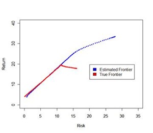
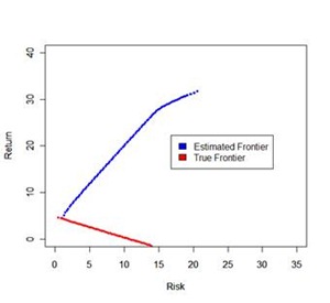
Using a few assets I looked at Estimated and True Frontier in two separate years, one in bull market and one in bear market. In the first illustration, the realized frontier is at least ok, but in the second case, the realized frontier shows pathetic results. It is not at all surprising that the frontier works well for minimum variance portfolios but falls flat for maximum return portfolio. This means “return forecast” is key to getting good performance for high risk profile investors.
Also, one can empirically check that errors in expected return are about 10 times more important than errors in covariance matrix, and errors in variance are twice more important than errors in covariance.
Shrinkage Estimators
One way to reduce the estimation error in the mean and covariance inputs is to follow either shrink the mean ( Jorion’s method) / shrink the cov( Ledoit and Wolf) method. I have tried the latter but till date have not experimented with shrinking both the mean and covariance at once. Can one do it ? I don’t know. Shrinking covariance towards a constant correlation matrix is what I have tried before. Estimator with no structure + Estimator with lot of structure + shrinkage intensity – These three components are essential for shrinkage of estimated mean. Ledoit and Wolf method shrinks the covariance matrix and compare the performance with sample covariance matrix, statistical factor model based on principal components, and a factor model. They find that shrinkage estimator outperforms other estimators for a global minimum variance portfolio.
Bayesian Approach via Black Litterman Model
Since expected returns are so much more important in the realized frontier performance, it might be better to use some model instead of sample mean as an input to the mean-variance framework. Black-Litterman model is one such popular model that combines views with prior distribution and gives the portfolio allocation for various risk profiles. If one has to explain Black-Litterman in words, it can be done this way – You want to strike a middle ground between market portfolio and “views”. You have an equation for market portfolio and you have an equation for views. You combine these equations and form a Generalized Linear Model, estimate the asset returns. These returns turn out to be a linear combination of market portfolio returns and expected return implied by investor’s views. One key thing to be understood is that you don’t have to views on all the assets in the considered asset universe. Even if you have views on few assets, that will change the expected return for all the assets.
However I am kind of skeptical about this method as I write. “Who in the world can give me views about the assets in the coming year?” If I poll a dozen people, there will more than dozen views with confidence intervals for their views. I have never developed a model with views till date. But as things change around me, it looks like I might have to incorporate views in to asset allocation strategies.
Part III of the book is a list about optimization techniques and appears more like a math book than a finance book .For an optimization-newbie, this chapter is not the right place to start. For an optimization-expert, the chapter will be too easy to go over. This chapter then is targeted towards a person who already knows quite a bit about optimization procedures and wants to know different viewpoints. Like most of the Fabozzi books that try to attempt at mathematical rigor and fail majestically, this part of the book throws not surprise. Part IV of the book talks about application of robust estimation and optimization methods.
 Takeaway :
Like many Fabozzi series books, the good thing about this book is that it has an extensive list of references to papers/ thoughts/opinions expressed by academia & practitioners about portfolio management. If the intention is to know what others have said/done in the area of portfolio management, then the book is worth going over.