An Introduction to Statistical Learning : Review

“Elements of Statistical Learning” (ESL) is often referred to as the “bible” for any person interested in building statistical models. The content in ESL is dense and the implicit prerequisites are good background in linear algebra, calculus and some exposure to statistical inference and prediction. Also, the visuals in ESL come with no elaborate code. If you don’t want to take them at face value and would like to check the statements / visuals in the book, you have got to sweat it out.

This book has four co-authors and two of them are coauthors of ESL, Trevor Hastie and Robert Tibshirani . Clearly the intent of the book is to serve as a primer to ESL. The authors have selected a few models from each of the ESL topics and have presented in such a way that anybody with an inclination to model can understand the contents of the book. The book is an amazing accomplishment by the authors as the book does not require any prerequisites such as linear algebra, calculus etc. Even the knowledge of R is not all that a prerequisite. However if you are not rusty with matrix algebra, calculus, probability theory , R etc., you can breeze through the book and get a fantastic overview of statistical learning.

I happened to go over this book after I had sweated my way through ESL. So, reading this book was like reiterating the main points of ESL. The models covered in ISL are some of the important ones from ESL. The biggest plus of this book is the generous visuals sprinkled throughout the book. There are 145 figures in a 440 page book, i.e. an average of one visual for every three pages. That in itself makes this book a very valuable resource. I will try to summarize some of the main points from ISL.

Introduction

Statistical Learning refers to a vast set of tools for understanding data. These tools can be classified as supervised or unsupervised. The difference between the two is that in the former, there is a response variable that guides the modeling effort whereas in the latter there is none. The chapter begins with a visual exploration of three datasets; the first dataset is wage data set that is used to explore the relationship between wage and various factors, the second data set is the stock market returns data set that is used to explore the relationship between the up and down days of returns with that of various return lags, and the third dataset is a gene expression dataset that serves an example of unsupervised learning. They try to summarize the gamut of statistical modeling techniques available for a modeler.There are 15 datasets used throughout the book. Most of them are present in ISL package on CRAN.

Some historical background for Statistical Learning

• 19th century - Legendre and Gauss method of least squares

• 1936 – Linear Discriminant Analysis

• 1940 – Logistic Regression

• 1970 – Generalized Linear Model - Nelder and Wedderburn

• 1980s – By 1980s computing technology improved Breiman, Friedman, Olshen and Stone introduced classification and regression trees. Also principles of cross-validation were laid out.

• 1986 – Hastie and Tibshirani coined the term generalized additive models in 1986 for a class of non-linear extensions to generalized linear models, and also provided a practical software implementation.

• In the recent years, the growth of R has made the availability of these techniques to a wide range of audience.

Statistical Learning

While building a model, it is helpful to keep in mind the purpose of the model. Is it for inferential purpose? Is it for prediction? Is it for both? If the purpose is to predict, then the exact functional form is not of interest as long as the prediction does a good job. If the model building is targeted towards inference, then exact functional form is of interest as it says a couple of things :

• What variables amongst the vast array of variables are important?

• What is the magnitude of this dependence?

• Is the relationship a simple linear relationship or a complicated one?

In the case of a model for inference, a simple linear model would be great as things are interpretable. In the case of prediction, non linear methods are good too as long as they give a good sense of predictability. Suppose that there is a quantitative response and there are p different predictors,[ . One can test out a model that build a relationship between [ and [ . The model would then be

where represents the systematic information that X provides about y.

The model estimate is represented by . There are two types of errors, one called the reducible error and the other called the irreducible error.

The above can further be broken down

So, whatever method you choose for modeling, there will be a seesaw between bias and variance. If you are interested in inference from a model, then linear regression, lasso, subset selection have medium to high interpretability. If you are interested in prediction from a model, then methods like GAM, Bagging, Boosting, SVM approaches can be used. The authors give a good visual that summarizes this tradeoff between interpretability and prediction for various methodologies.

The following visual summarizes the position of various methods on bias variance axis.

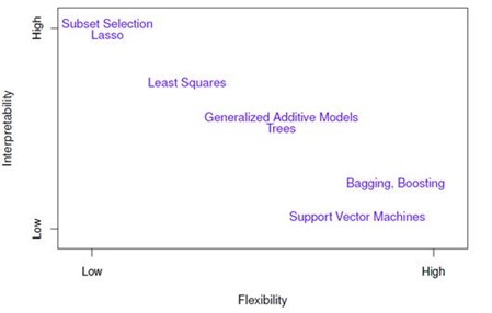
When inference is the goal, there are clear advantages to using simple and relatively inflexible statistical learning methods. In some settings, however, we are only interested in prediction, and the interpretability of the predictive model is simply not of interest. Like in the case of an algo trading model, it does not matter what the exact form of the model is as long as it is being able to predict the moves correctly. There is a third variation of learning besides the supervised and unsupervised learning. Semi supervised learning is where you have response variable data for a subset of your entire data but is not present for the rest of data.

The standard way to measure model fit is via mean squared error

This error is typically less on training dataset. One needs to check the statistic on the test data and choose that model that gives the least test MSE. There is no guarantee that the method that has the least error on the training data will also have the least error on the test data.

I think the following statement is the highlight of this chapter:

Irrespective of the method used, as the flexibility of the method increases, it results in a monotonically decreasing error for the training data and U shaped curve for the test data for the test data

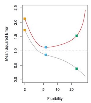
Why do we see an inverted U curve? As more flexible methods are explored, variance will increase and bias will go down. As you start with more flexible methods, the bias starts to decrease more than the increase in variance. But beyond a point, the bias hardly changes and variance begins to increase. This is the reason for the U curve for the test MSE.

In the classification setting, the golden standard for evaluation is the conditional probability

for various classes. This simple classifier is called the Bayesian classifier. The Bayes classifier’s prediction is determined by the Bayes decision boundary. The Bayes classifier provides the lowest possible rate. Since the Bayes classifier will always choose the class for which the conditional probability is the largest, the error rate has a convenient form.The Bayes error rate is analogous to the irreducible error. This connection between Bayes error rate and irreducible error is something that I had never paid attention to. For real data, one does not know the conditional probability. Hence computing Bayesian classifier is impossible. In any case Bayes classifier stands as the gold standard against which to compare methods, for simulated data. If you think about the K nearest neighbor methods, as the number of neighbors increases, the bias goes up and variance goes down. For a neighbor of size 1, there is no bias but a lot of variance. Thus if you are looking for a parameter to characterize the increasing flexibility, then 1/K is a good choice. Typically you see a U curve for the test data and then you can zoom in on to the K value that yields minimum MSE.

Linear Regression

This chapter begins with a discussion about the poster boy of statistics, linear regression. Why go over linear regression? The chapter puts it aptly,

Linear regression as a good jumping off point for newer approaches.

This chapter teaches one to build a linear models with hardly mention on linear algebra. Right amount of intuition and right amount of R code drives home the lesson. A case in point is illustrating the case of spurious regression via this example:

Assuming that you are investigating shark attacks. You have two variables ice cream sales and temperature. If you regress shark attacks with ice cream sales, you might see a statistical relationship. If you regress shark attacks with temperature, you might see a statistical relationship. If you regress shark attacks with ice cream sales and temperature, then you might see ice cream sales variable being knocked off? Why is that?

Let’s say there are two correlated predictors and one response variable. If you regress the response variable with each of the individual predictors, the relationship might show a statistically significant relationship. However if you include both the predictors in a multiple regression model, one might see that only one of the variables is significant. In a multiple regression scenario, some of the correlated variables get knocked off for the simple reason that the effect of the predictor is measured keeping all else constant. If you want to estimate the coefficient of ice cream sales, you keep the temperature constant and check the relationship between the shark attacks and ice cream sales. You will immediately see that there is no relationship whatsoever. This is a nice example (for class room purpose) that drives home the point that one must be careful about correlation between predictors.

Complete orthogonality amongst predictors is an illusion. In reality, there will always be a correlation between predictors. What are assumptions behind a linear model?. Any simple linear models has two assumptions, one being additivity, the other being linearity. In additivity assumption, the effect of changes in a predictor on the response [ is independent of the values of the other predictors.In linearity assumption, the change in the response [ due to a one-unit change in [ is constant, regardless of the value of [.

Why are prediction intervals wider than confidence intervals ? Something that is not always given a nice explanation in words. The chapter puts it nicely. Given a model you will be able to predict the response up to irreducible error. What this means is that even if you know the true population parameters, you model says that there is an irreducible error. You can’t escape this error. For a given set of covariates, one can form two sets of confidence bands. The first type of confidence bands is called confidence intervals where the bands are for training data. The prediction interval is wider than the confidence interval as it also includes the systematic error. Confidence interval tells what happens on an average whereas prediction interval tells what happens for a specific data point.

Basic inference related questions

• Is at least one of the predictors useful in predicting response ? The classic way to test this do an anova so that it throws the relevant statistic. The summary table of the linear regression reports p values that are partialled out effects. So, in the contexts of fewer predictors, it is ok to see the pvalue and be happy with it. However if there are large number of predictors, by sheer randomness some of the coefficients can show statistical relationship. In all such cases, one needs to look at the F statistic.

• Do all the predictors help explain ? Forward selection, Backward selection or Hybrid methods can be used.

• How well does the model fit the data Mallows , AIC, BIC, Adjusted [. These are all the metrics that give an estimate of test error based on training error

• Given a set of predictors, what response values should we predict and how accurate is our prediction?

Clearly there are a ton of aspects that go wrong when you fit real life data, some of them are :

• Non linearity of the response-predictor relationships - Residual Vs Fitted plots might give an indication of this. transforming the independent variables can help.

• Correlation of error terms: In this case the error matrix has a structure and hence you can use generalized least squares to fit a model. Successive terms can be correlated. This means that you have to estimate the correlation matrix if truly has that assumed correlation This is an iterative procedure. Either you can code it up or conveniently use nlme package.

• Non constant variance of error terms - If you see a funnel shaped graph for variance of error terms, then a log transformation of response variable can be used

• Outliers in the model bloat the RSE and hence all the interpretations of confidence intervals become questionable - Plot studentized residuals to cull out outliers

• High Leverage points : Outliers are more relevant to unusual response variable values where leverage points are unusual covariate data points.There are standard diagnostic plots to identify these miscreants.

• Collinearity : Because of collinearity, for similar value of RSS, different estimates of coefficients can be chosen. The joint distribution is a narrow valley and hence the parameter estimates are very unstable. This basically has to do with design matrix not being a full column rank. might be almost singular matrix. Hence some of the eigen values of the matrix could be very close to 0. Hence the best way to understand collinearity is to compute variance inflation factor. faraway package has a function vif that automatically gives vif for all the predictors. Well , nothing much can be done to reduce the collinearity as the data has already been collected. All one can do is to drop the collinear column or take a linear combination of such columns and replace the columns by a single column.

The chapter ends with a section on KNN regression. KNN regression is compared with linear regression to comment on the non parametric vs. parametric modeling approaches. KNN regression works well if the true model is non linear. But if the number of dimensions increases, this method falters. Using the bias variance trade off graph for training and test data given in the chapter , one can see that KNN performs badly if the true data is linear and K is small. If K is very large and the true model is linear, then KNN method works as well as a parametric model.

The highlight of this chapter as well as this book is readily available visuals that are given to the reader. All you have to do is study them . If you start with ESL instead of this book, you have to not only know the ingredients but also code it up and check all the statements for yourself. This book makes life easy for the reader.

Classification

I sweated through the chapter on classification in ESL. May be that’s why, I found this chapter on classification a welcome recap of all the important points and in fact a pleasant experience to read through. The chapter starts off with illustrating the problem of using a linear regression for a categorical variable. Immediately it shows that a variation of linear model, i.e. logit model . However if the categorical variable has more than 2 levels, then the performance of multinomial logit starts to degrade.

The chapter gives a great example of paradox. The dataset used to illustrate this is the one that contains default rate, credit card balances, income and a categorical variable student. If you regress the default rate against student variable, you find that the variable is significant. If you regress default rate with balance and student variable, the student variable is kicked out. This is similar to shark attacks-temperature-ice-cream sales case. There is an association between the balance and default rate. The fact that student comes up as a statistically significant variable is due to the fact that the student variable is correlated with balance variable. Here is a nice visual to illustrate confounding.

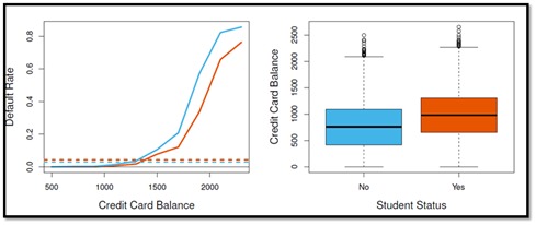
Visual on the left says at any given level the default rate of student is less than that of non-student. However average default rate of student is more than the average default rate of non-student. This is mainly because of the confounding variable. If you look at the visual on the right, the students typically carry a lot of balance and that is variable that is driving the default rate. The conclusions from this is : On an average students are risky than non-students if you don’t have any information. But given a specific balance, the default rate of non-students is more than students. I am not sure but I think this goes by the name of `` Simpson’s Paradox''

In cases where there are more than two levels for the categorical variable, it is better to go for a classification techniques. What’s the basic idea? You model the distribution of the predictors X separately in each of the response classes and then use Bayes to flip these around in to estimates for posterior probabilities of the response variable belonging to a specific class. LDA and QDA are two popular techniques for classification. LDA assumes a common covariance structure of the predictors for each of the separate levels of the response variable. It then uses Bayes to come up with a linear discriminant function to bucketize each observation. Why prefer LDA to Logistic in certain cases?

• When the classes are well-separated, the parameter estimates for the logistic regression model are surprisingly unstable. LDA does not suffer from this problem

• If sample size is small and the distribution of the predictors is approximately normal in each of the classes, the LDA is again more stable than logistic regression model

• LDA is popular when there are more than two responses

QDA assumes separate covariance matrix for each class and is useful when there is a lot of data and variance is not of great concern. In LDA, one assumes same covariance matrix and such an assumption is useful when the dataset is small and there is a price to pay for estimating parameters. If sample size is small LDA is a better bet than QDA. QDA is recommended if the training set is large, so that the variance of the classifier is not a major concern

There are six examples that illustrate the following points

• When the true decision boundaries are linear, then LDA and logistic regression approaches will tend to perform well

• When boundaries are moderately non-linear, QDA may give better results

• For much more complicated boundaries, a non parametric approach such as KNN can be superior. But the level of smoothness for non parametric method needs to be chosen carefully.

• Ideally one can think of QDA as the middle ground between LDA and KNN type methods

The lab at the end of the chapter gives the reader R code and commentary to fit logit models, LDA model, QDA model, knn model. As ISL is a stepping stone for ESL, it is not surprising that many other aspects of classification are not mentioned. A curious reader can find regualarized discriminant analysis, connection between QDA and Fischer’s discriminant analysis and many more topics in ESL. However in the case of ESL, there is no spoon feeding. You have to sweat it out to understand. In ESL, there is a mention of an important finding. Given that LDA and QDA make such a harsh assumption on the nature of the data, it is surprising to know that they are two most popular practitioner’s methods.

Resampling Methods

This chapter talks about Resampling methods, the technique that got hooked me on to statistics. It is an indispensable tool in modern statistics. This chapter talks about two most commonly used resampling techniques : cross-validation and bootstrap

Why cross-validation ?

• Model Assessment : It is used to estimate the test error associated with a given statistical learning method in order to evaluate its performance.

• Model Selection : Used to select the proper level of flexibility. Let’s say you are using KNN method and you need to select the value of K. You can do a cross validation procedure to plot out the test error for various values of K and then choose the K that has the minimum test error rate.

The chapter discusses three methods, one being validation set approach, the second one being LOOCV( Leave one out cross validation ) and k-fold cross validation method. In the first approach, a part of data set is set aside for testing purpose. Flexibility parameter is chosen in such a way that MSE is minimum for that level of flexibility.

What’s the problem with Validation set approach?

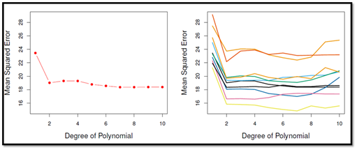
• There are two problems with validation set approach. The test error estimate has a high variability as it depends on how you choose your training and test data. Also in the validation set approach, only part of the data is used to train the model. Since the statistical methods tend to perform worse when trained on fewer observations, this suggests that the validation set error rate may tend to overestimate the test error rate.

• LOOCV has some major advantages. It has less bias. It uses almost the entire data set. It does not overestimate the test error rate. With least square or polynomial regression, LOOCV has an amazing formula that cuts down the computational time. It is directly related to hat values and residual values. But there is no readymade formula for other models and thus LOOCV can be computationally expensive. As an aside if you use LOOCV to choose the bandwidth in Kernel density estimation procedure, all the hard work of that FFT does is washed away. It is no longer O(n log n).

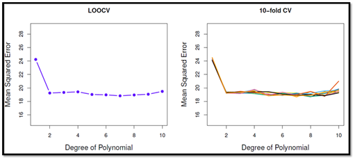
• k fold CV is far better from a computational stand point. It has some bias as compared LOOCV but it has lesser variance that LOOCV based estimate. So, in the gamut of less bias more variance- more bias less variance, a 5 fold CV or a 10 fold CV has been shown to yield test error rates that do not suffer from excessively high bias or high variance.

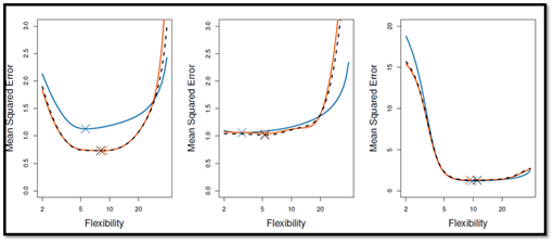
Most of the times we does not have the true error rates. Nor do we have the Bayesian boundary. We are testing out models with various flexibility parameters. One way to choose the flexibility parameter is to estimate test error rate using k fold CV and choose the flexibility parameter that has the lowest test error rate. As I have mentioned earlier, the visuals are the highlight of this book.

The following visual shows the variance of test error estimate via validation set method

The following visual shows the variance of test error estimate via k fold CV. The variance of estimate is definitely less than validation method

The following visual shows the selecting a flexibility parameter based on LOOCV or k fold CV will yield almost similar results

The chapter ends with an introduction to bootstrap, a method that samples data from the original data set with replacement and repeatedly computes the desired parameters. This results in a realization of the parameter sample from which standard error of the parameter can be computed.

I learnt an important aspect of bootstrapping. The probability that a specific data point is not picked up in bootstrapping is 1/e. This means that even though you are bootstrapping away to glory, there are 1/3 of the observations that are not touched. This also means that when you try to build a model on one bootstrapped sample, you can actually test that model on the 1/3 of observations that haven’t been picked up. In fact this is exactly the idea that is used in bagging, a method to build regression trees. Well, you can manually write the code for doing cross validation, be it LOOCV or k fold CV. But R gives all of them for free. The lab mentioned at the end of the chapter talks about boot package that has many functions that allow you do to cross validation directly. In fact after you have worked with some R packages , you will realize that most of the packages have the cross validation argument in the modeling functions as it allows the model to pick the flexibility parameter based on k fold cross validation

After going through R code from the lab, I learnt that it is better to use subset argument in building a model on a subset of data. I was following a painful process of actually splitting the data in to test and trained sample. Instead one can put in the index of observations that are meant for training data, and model will be built on those observations only. Neat!

Linear Model Selection and Regularization

Alternative fitting procedures to least squares can yield better prediction accuracy and model interpretability. If there is no unique least squares coefficient. However shrinking the estimated coefficients, one can substantially reduce the variance of the coefficients, at the cost of a negligible increase in bias. Also least squares usually fits all the predictors. There are methods that help in the feature or variable selection.

There are three alternatives to least squares that are discussed in the book.

• Subset Selection : Identify a subset of predictors that we believe to be related to the response

• Shrinkage : Regularization involves shrinking the coefficients and depending on the method, some of the shrinkage coefficients can be 0, thus making it a feature selection method

• Dimension Reduction : This involves projecting the predictors on to a [ dimensional space with [

In the Best subset selection, you choose amongst models. Since this is computationally expensive, one can use forward / backward or hybrid methods. The number of models fitted in a forward / backward regression model is [ How does one choose the optimal model? There are two ways to think about this. Since all the models are built on a dataset and that’s all we have, we can adjust the training error rate as it usually a poor estimate of test error rate. So, there are methods like Mallows [, AIC, BIC, Adjusted [. All these results are obtained via regsubsets function from the leaps package.

The other method is via Validation and Cross validation. Validation method involved randomly splitting the data and training the data on one set and testing the trained model on the test dataset. The model that gives the least test error is chosen. K fold cross validation method means splitting the data in to k segments, training the model using k-1 segments and testing it out on the held out segment and redoing this k times and then averaging out the error. Both these methods give a direct estimate of the true error and do not make distributional assumptions. Hence these are preferred over methods that adjust training error. An alternative to best subset selection is a class of method that penalizes the values the predictor coefficients can take. The right term to use is “regularizes the coefficient estimates”. There are two other methods discussed in the text, one being ridge regression and other being lasso. The penalizing function is an penalty for ridge regression whereas it is [ penalty for lasso.

The math behind the three types of regression can be succinctly written as

Ridge regression

lasso regression

Best subset regression

Some basic points to keep in mind

• One should always standardize the data. For least square the estimates are scale invariant. But ridge regression and lasso are dependent on and the scaling of the predictor.

• Ridge regression works best where the least squares estimate have high variance. In Ridge regression none of the coefficients have exactly 0 value. In lasso, the coefficients are taken all the way to 0. Lasso is more interpretable than Ridge regression.

• Neither Ridge nor Lasso universally dominate the other. It all depends on the true model. If there are small number of predictors and the rest of predictors have small coefficients lasso performs better than ridge. If the modeling function is dependent on many predictors, then ridge performs better than lasso.

• The best way to remember lasso and ridge is that lasso shrinks the coefficients by the same amount whereas ridge shrinks the coefficients by the same proportion. In either case the best way to choose the regularization parameter is via cross validation.

• There is Bayes angle to the whole discussion on lasso and ridge. If you think from a Bayesian point of view, lasso is like assuming a Laplace prior for betas where ridge is like assuming a Gaussian prior for betas

The other method that is discussed in the chapter fall under dimension reduction methods. The first such method is Principal component regression. In this method, you create various linear combination of predictors in such a way that each of the components has maximum variance of the data. All dimension reduction methods work in two steps. First, the transformed predictors are obtained. Second, the model is fit using these [ predictors. There are two ways to interpreting PCA directions. One is the direction along which the data shows the maximum variance. The second way to interpret is the directions along which the data points are closest.

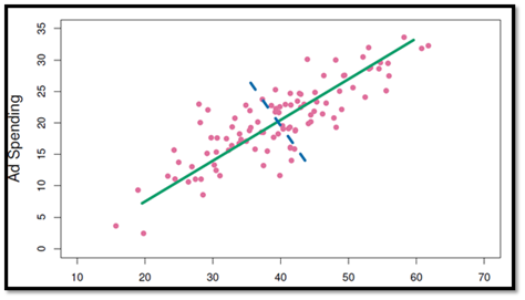
What does this visual say ? By choosing the right direction, one gets the predictors having maximum variance in this direction. This means the coefficients are going to be more stable if there is maximum variance shown by the predictor. The standard error of is [ . In all the cases when predictors are close, the standard errors are bloated. By choosing the directions along the principal components, standard error of [ is low.

Observe these visuals

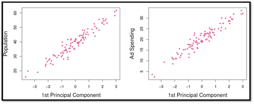
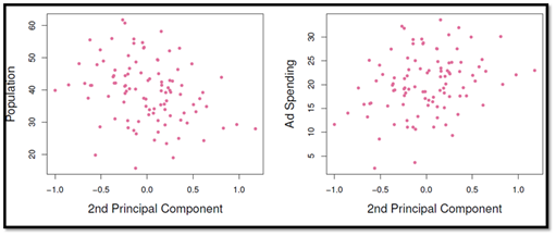
The first component captures most of the information that is present in the two variables. The second principal component has nothing much to contribute. By regressing using these principal components, the standard errors of betas are less,i.e., the coefficients are stable. Despite having gone through Partial least squares regression in some of the previous texts, I think the following visual made all come together for me.

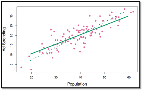
This shows the PLS based regression chooses a slightly tilted direction as compared to PCR. The reason being, the component directions are chosen in such a way that the response variable is also taken in to consideration. The best way to verbalize PCLS is that it is a “supervised alternative” to PCR. The chapter gives the basic algo to perform PLS

Towards the end of the chapter, the book talks about high dimensional data where . Data sets containing more features than observations are often referred to as high-dimensional. In such a dataset, the model might overfit. Imagine fitting a linear regression model with 2 predictors and 2 observations. It will be a perfect fit and hence residuals will be 0 and the [ will be 100%. When [ , a simple least squares regression line is too flexible and hence overfits the data.

Your training data might show that one should use all the predictors, but all it says that it is just fitting one model out of a whole lot of models to describe the data. How to deal with high dimensional data? Forward stepwise selection, ridge regression, lasso, and principal component regression are particularly useful for performing regression in the high dimensional setting. Despite using these three methods, there are three things that need to be kept in mind

• Regularization or shrinkage plays a key role in high-dimensional problems

• Appropriate tuning parameters selection is crucial for good predictive performance

• The test error tends to increase as the dimensionality of the problem increases, unless the additional features are truly associated with the response

Another important thing to be kept in mind is in reporting the results of high-dimensional data analysis. Showing training

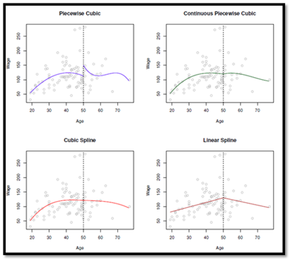
In the top left , you specify unconstrained cubic polynomials. In the top right, you impose a constraint of continuity at the knot. In the bottom left you impose a constraint on continuity, the first derivative and the second derivative. A cubic spline uses a total of degrees of freedom. A degree-d spline, is one that is piecewise degree-d polynomial, with continuity in derivatives up to degree d-1 at each knot. Fitting regression spline can be made easy by fitting a model with truncated power basis function per knot. 

To cut the variance of splines, one can use another constraint at the boundary that results in natural splines. 

What’s the flip side of Local Regression ? Local regression can perform poorly if number of predictors is more than 3 or 4. This is the same problem that KNN suffers from in the case of high dimensionality.

The chapter ends with GAM (Generalized Additive Models) that provide a general framework for extending a standard linear model by allowing non-linear functions of each of the variables, while maintaining additivity.

There are a ton of functions mentioned in the lab section that equips a reader to estimate the parameters of  polynomial regression models, cubic splines, natural spline, smoothing spline, local regression etc..

Tree Based Methods

What’s the basic idea? Trees involve stratifying or segmenting the predictor space in to a number of simple regions. In order to make a prediction, one typically uses the mean or the mode of the training observations in the region to which it belongs. Tree based methods are simple and useful for interpretation. However they are not competitive with the best supervised learning approaches. Hence a better alternative is creating multiple trees and then combining all of them in one big tree.

The chapter starts with Decision trees. These can be applied to both regression and classification tasks. In regression task, the response variable is continuous whereas in classification, the response variable is discrete. In the case of regression trees, the predictor space is split into distinct and non-overlapping regions [ . The goal is to find boxes such that

where the mean response rate within the jth box. To make it computationally practical, a recursive binary splitting method is followed. A top-down greedy algorithm is used. At each step the best split is made at that particular step, rather than looking ahead and picking a split that will lead to a better tree in some future step. The problem with this approach is that the fitted tree could be too complex and hence it might perform poorly on the test data set. To get over this problem, one of the approaches is to build the tree and then prune the tree. This is called Cost complexity pruning. The way this is done is similar to lasso regression.

Classification tree is similar to a regression tree, except that it is used to predict a qualitative response rather than a quantitative response. Since one is not only interested in the class prediction for a particular terminal node, but also the class proportions among the training observations that fall in to the region. RSS cannot be used. What one needs to use classification error rate. The classification error rate is simply the fraction of the training observations in that region that do not belong to the most common class. There are two other metrics used for splitting purposes (measures of node purity)

• Gini Index

• Cross-entropy index

The key idea from this section is this :

One can fit a linear regression model or a regression tree. The relative performance of one over the other depends on the underlying true model structure. If the true model is indeed linear, then linear regression is much better. But if the predictor space is non linear, it is better to go with regression tree. Even though trees seem convenient for a lot of reasons like communication, display purposes etc., the predictive capability of trees is not all that great as compared to regression methods.

The chapter talks about bagging, random forests and boosting, each of which are dealt at length in ESL. Sometimes I wonder whether it is better to understand a topic in depth before getting an overview of it or the other way round. The problem with decision trees is that it is has high variance. If the training and test data are split in a different way, a different tree is built. To cut down the variance, bootstrapping is used. You bootstrap the data, create a tree and aggregate against all the bootstrapped trees.

There is a nice little fact mentioned in one of the previous chapters that says that the probability of a data point that is not selected in a bootstrapping exercise approaches e. Hence for every bootstrap, there are 1/3rd of the training points that are not selected for tree formation. Once the tree is formed for that bootstrapped sample, these Out of bag sample can be tested and over multiple bootstraps, you can form an error estimate based for every observation. A tweak on bagging that decreases the correlation between the bootstrapped trees is random forests. You select at random a set of parameters; build a tree and then average over many such boot strap samples. The number of predictors chosen is typically square root of the number of parameters. The chapter also explains Boosting that is similar to bagging but learns slowly.

Unsupervised Learning

This chapter talks about PCA and clustering methods. At this point in the book, i.e. towards the end of the book, I felt that it is better to sweat it out with ESL and subsequently go over this book. The more one tries to sweat it out with ESL , the more ISL will turn out to be a pleasant read.. May be I am biased here. May be the right way could ISL to ESL. Whatever be the sequence, I think this book will serve as an apt companion to ESL for years to come.