Percentage times reverted
\maketitle
This is an improvement to the pairs algorithm. Basically , it involves taking any 15 day time period and checking whether the spread sigma < 0.4
> x <- security.db1[, c("UNIONBANK", "PNB")]
> gamma <- 0.241924965
> intercept <- 52.555924557
> spread.mean <- -0.422750321
> spread.sigma <- 11.647152896
> spread.level <- (x[, 1] - gamma * x[, 2] - intercept - spread.mean)/spread.sigma
> N <- 1e+05
> indices <- round(runif(N, 1, 215), 0)
> reverted <- 0
> i <- 1
> for (i in 1:N) {
+     start <- indices[i]
+     end <- indices[i] + 15
+     if (length(which(abs(spread.level[start:end]) < 0.4)) > 1)
+         reverted <- reverted + 1
+ }
> reverted/N
[1] 0.75921 |
This shows that there is 75 percentage probability that the spread will revert Another related work that I want to do is to develop a probit model
> nifty <- read.csv("nifty.csv", header = T)
> par(mfrow = c(2, 1))
> plot(spread.level, type = "l", col = "blue")
> plot(nifty[, 1], type = "l", col = "blue") |
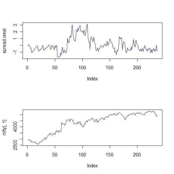
Basic idea If we take the example of UNIONBANK-PNB, if you put on a position, the spread can converge in its lifetime else not. Historically the spread would have diverged in a specific time slot or converged in a time slot. It could have some relationship with NIFTY movement. So, the fact that spread converges in a specific # of days could be a dependent variable Yt . Yt takes the value of 1 if the spread converges. Else it takes the value of 0.
Thus the dependent variable is Yt (1/0). Independent variable could be NIFTY movement . Havent thought through this properly