Poisson
Purpose I was working on Poisson today and I could not help but wonder at the things that I do not know anything absolutely. Some of the basic things I did not have a clue about.
After living for 33 years, I was completely ignorant about so many things that I am embarassed. What was I doing all these years ? Did I do anything worthwhile in my life..
Ok, tossing these philosophical questions aside, here are some of the learnings - Probability Generation Function. This is a succinct way of representing the entire discrete prob function in one specific way. - Mean and Variance for a poisson are same . However in reality, it usually never is the case. - A month ago if anyone would have asked me to prove that in the limit, you can approximate binomial with poisson, I would have failed big time. Today I learnt that using a simple recursive relation, you can prove it - for K > Lambda and K>1 , the probs go up and then go down peaking at K - for Lambda < 1 , the probs show a decreasing tendency - When you build a poisson regression model, the issues of heteroscedasticity becomes very very important. This issue of heteroscedasticity can be handled with dispersion function. This dispersion function gives no reduction in the estimate values but gives a redution in the standard errors associated with the estimates.
ok, that makes me think about something..getting estimates with lesser standard error is much better than getting estimates with higher standard error.
coming back to testing poisson
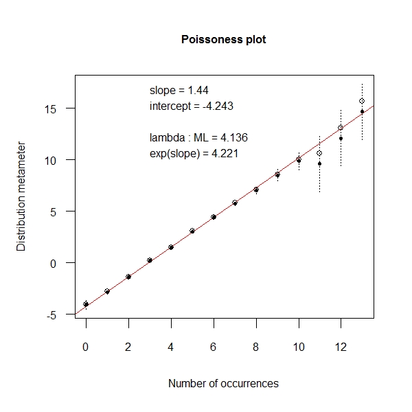
Book Visualizing Categorical data provides a means to test the poissonness of the data. Well the underlying logic is extremely simple. Refer to the book. At its heart , it is a simple regression which helps you decide whether the data is from a poisson distribution
> x <- rpois(1000, 4) > distplot(x, type = "poisson") |
Another way is to use ChiSquare distribution
> z <- table(x) > z <- as.data.frame(cbind(as.numeric(names(z)), z)) > z1$expected <- 1000 * ppois(z1[, 1], 4) > crit <- sum((z1[, 2] - z1[, 3])^2/(z1[, 3])) > dchisq(crit, 10) [1] 0 |
Thus you can reject the alternate hypo that the underlying distributions for the data is different