Granger Test Vs ECM

Purpose The purpose is to explore the unstability arising from structural change in the time series data. Till this point in time, I was merely analyzing the timeseries data with out any consideration of structural shift

I am using a different script to generate the dataset needed for testing the structural shifts in pairs data.

Basic steps :

Shortlist the pairs

> library(fArma)
> library(fSeries)
> library(TSA)
> library(pspline)
> library(fUnitRoots)
> library(RSQLite)
> library(lmtest)
> program.date <- "feb18"
> ticker.data <- "tickers.csv"
> date.start <- "2009-02-02"
> date.end <- "2010-02-18"
> setwd("C:/Cauldron/garage/R/soulcraft/Data/Pairs")
> source("C:/Cauldron/garage/R/soulcraft/Volatility/Pairs/RelativeValue/ZCT.R")
> INITIAL.CAPITAL <- 1e+06
> UNITS <- 1e+05
> all.pairs.file <- paste("all_pairs_", program.date, "_v1.csv",
+     sep = "")
> shortlisted.pairs.file <- paste("shortlisted_pairs_", program.date,
+     "_v1.csv", sep = "")
> arma.file <- paste("arma_", program.date, "_revised.csv", sep = "")
> final.pairs.file <- paste("finalpairs_", program.date, ".csv",
+     sep = "")
> discuss.pairs.file <- paste("disusspairs_", program.date, ".csv",
+     sep = "")
> eacf.result.file <- paste("eacf_resultfile_", program.date, ".csv",
+     sep = "")
> db <- "C:/sqlite/mydbases/pairs/pairsv1.s3db"
> drv <- dbDriver("SQLite")
> con <- dbConnect(drv, dbname = db)
> query <- paste("') \n\t\t\t\t\t\t\t\torder by ticker_id, trade_date asc ",
+     sep = "")
> security.db <- dbGetQuery(con, query)
> security.db <- security.db[, 3:4]
> security.db1 <- unstack(security.db, form = security.db$price ~
+     security.db$ticker)
> stkreturns <- returns(ts(security.db1), "simple")
> stkreturns <- stkreturns[-1, ]
> n <- dim(stkreturns)[2]
> pair.combinations <- matrix(data = NA, nrow = n * (n + 1)/2,
+     ncol = 2)
> rowcount <- 1
> for (i in 1:n) {
+     for (j in 1:i) {
+         pair.combinations[rowcount, 1] <- i
+         pair.combinations[rowcount, 2] <- j
+         rowcount <- rowcount + 1
+     }
+ }
> pair.combinations <- data.frame(pair.combinations)
> colnames(pair.combinations) <- c("i", "j")
> lookupi <- tickers[, c("tickers", "ticker_id", "mktcap.cr", "sector",
+     "sector_id")]
> lookupj <- tickers[, c("tickers", "ticker_id", "mktcap.cr", "sector",
+     "sector_id")]
> colnames(lookupi) <- c("tickeri", "i", "mktcap.cr.i", "sector.i",
+     "sector.i.id")
> colnames(lookupj) <- c("tickerj", "j", "mktcap.cr.j", "sector.j",
+     "sector.j.id")
> d1 <- merge(pair.combinations, lookupj, by.x = "j", by.y = "j",
+     all.x = T)
> d2 <- merge(d1, lookupi, by.x = "i", by.y = "i", all.x = T)
> d3 <- d2[d2$i != d2$j, c("i", "j", "tickeri", "tickerj", "sector.i",
+     "mktcap.cr.i", "sector.j", "mktcap.cr.j", "sector.i.id",
+     "sector.j.id")]
> samesector <- d3[d3$sector.i.id == d3$sector.j.id, ]
> x <- pmax(samesector$mktcap.cr.i, samesector$mktcap.cr.j)/pmin(samesector$mktcap.cr.i,
+     samesector$mktcap.cr.j)
> x <- round(x, 0)
> cumsum(table(x)) * 100/sum(table(x))
        1         2         3         4         5         6         7         8
 20.51282  37.94872  52.30769  61.53846  68.20513  74.10256  77.69231  79.74359
        9        10        11        12        13        14        15        16
 81.02564  82.82051  84.61538  85.12821  86.41026  86.92308  87.94872  88.71795
       17        18        19        21        22        23        24        25
 89.48718  90.00000  91.02564  92.05128  93.07692  93.58974  94.10256  94.61538
       26        27        28        29        31        33        36        45
 95.12821  95.38462  95.64103  95.89744  96.15385  96.66667  96.92308  97.17949
       49        51        55        60        64        69        75        84
 97.43590  97.94872  98.20513  98.46154  98.71795  98.97436  99.23077  99.74359
       87
100.00000
> samesector <- samesector[which(x <= 8), ]

> sector.tests <- samesector
> sector.tests$p.a.b.1 <- 0
> sector.tests$p.a.b.2 <- 0
> sector.tests$p.a.b.3 <- 0
> sector.tests$p.b.a.1 <- 0
> sector.tests$p.b.a.2 <- 0
> sector.tests$p.b.a.3 <- 0
> sector.tests$lag.coeff.a.b <- 0
> sector.tests$lag.coeff.b.a <- 0
> sector.tests$p.a.b.3.W <- 0
> sector.tests$p.b.a.3.W <- 0
> npairs <- dim(samesector)[1]
> pair = 1
> for (pair in 1:npairs) {
+     a <- samesector[pair, "tickeri"]
+     b <- samesector[pair, "tickerj"]
+     y1 <- (security.db1[, a])
+     x1 <- (security.db1[, b])
+     p.a.b.3.W <- (grangertest(y1 ~ x1, order = 1))[2, 4]
+     y1 <- log(security.db1[, a])
+     x1 <- log(security.db1[, b])
+     fit <- lm(y1 ~ x1)
+     if (summary(fit)$coefficients[1, 4] < 0.05) {
+         error <- residuals(fit)
+     }
+     else {
+         fit <- lm(y1 ~ x1 + 0)
+         error <- residuals(fit)
+     }
+     n <- length(error)
+     res <- unitrootTest(error, lag = 1, type = "c")
+     p.a.b.1 <- attr(res, "test")$p.value[1]
+     dy1 <- diff(y1)
+     dx1 <- diff(x1)
+     error.lag <- error[-n]
+     fit <- lm(dy1 ~ error.lag + dx1)
+     fit.summary <- summary(fit)
+     p.a.b.2 <- fit.summary$coefficients[2, 4]
+     z <- data.frame(embed(cbind(dy1, dx1), 2))
+     colnames(z) <- c("dy1", "dx1", "dy1.1", "dx1.1")
+     error.lag <- error[-c(1, n)]
+     fit <- lm(dy1 ~ error.lag + dy1.1 + dx1.1, data = z)
+     fit.summary <- summary(fit)
+     p.a.b.3 <- fit.summary$coefficients[2, 4]
+     lag.coeff.a.b <- fit.summary$coefficients[2, 1]
+     y1 <- (security.db1[, b])
+     x1 <- (security.db1[, a])
+     p.b.a.3.W <- (grangertest(y1 ~ x1, order = 1))[2, 4]
+     y1 <- log(security.db1[, b])
+     x1 <- log(security.db1[, a])
+     fit <- lm(y1 ~ x1)
+     if (summary(fit)$coefficients[1, 4] < 0.05) {
+         error <- residuals(fit)
+     }
+     else {
+         fit <- lm(y1 ~ x1 + 0)
+         error <- residuals(fit)
+     }
+     n <- length(error)
+     res <- unitrootTest(error, lag = 1, type = "c")
+     p.b.a.1 <- attr(res, "test")$p.value[1]
+     dy1 <- diff(y1)
+     dx1 <- diff(x1)
+     error.lag <- error[-n]
+     fit <- lm(dy1 ~ error.lag + dx1)
+     fit.summary <- summary(fit)
+     p.b.a.2 <- fit.summary$coefficients[2, 4]
+     z <- embed(cbind(dy1, dx1), 2)
+     colnames(z) <- c("dy1", "dx1", "dy1.1", "dx1.1")
+     error.lag <- error[-c(1, n)]
+     fit <- lm(z[, "dy1"] ~ error.lag + z[, "dy1.1"] + z[, "dx1.1"])
+     fit.summary <- summary(fit)
+     p.b.a.3 <- fit.summary$coefficients[2, 4]
+     lag.coeff.b.a <- fit.summary$coefficients[2, 1]
+     sector.tests[pair, "p.a.b.1"] <- p.a.b.1
+     sector.tests[pair, "p.a.b.2"] <- p.a.b.2
+     sector.tests[pair, "p.a.b.3"] <- p.a.b.3
+     sector.tests[pair, "p.b.a.1"] <- p.b.a.1
+     sector.tests[pair, "p.b.a.2"] <- p.b.a.2
+     sector.tests[pair, "p.b.a.3"] <- p.b.a.3
+     sector.tests[pair, "lag.coeff.a.b"] <- lag.coeff.a.b
+     sector.tests[pair, "lag.coeff.b.a"] <- lag.coeff.b.a
+     sector.tests[pair, "p.a.b.3.W"] <- p.a.b.3.W
+     sector.tests[pair, "p.b.a.3.W"] <- p.b.a.3.W
+ }

There are 6 categories which I want to explore

> dim(sector.tests)
[1] 311  20
> temp <- sector.tests[, c("p.a.b.1", "p.a.b.2", "p.a.b.3", "p.b.a.1",
+     "p.b.a.2", "p.b.a.3", "p.a.b.3.W", "p.b.a.3.W", "lag.coeff.a.b",
+     "lag.coeff.b.a")]
> temp$stat.a.b.1 <- ifelse(temp$p.a.b.1 < 0.05, 1, 0)
> temp$stat.b.a.1 <- ifelse(temp$p.b.a.1 < 0.05, 1, 0)
> temp$stat.a.b.2 <- ifelse(temp$p.a.b.2 < 0.05, 1, 0)
> temp$stat.b.a.2 <- ifelse(temp$p.b.a.2 < 0.05, 1, 0)
> temp$stat.a.b.3 <- ifelse(temp$p.a.b.3 < 0.05, 1, 0)
> temp$stat.b.a.3 <- ifelse(temp$p.b.a.3 < 0.05, 1, 0)
> temp$stat.a.b.3.W <- ifelse(temp$p.a.b.3.W < 0.05, 1, 0)
> temp$stat.b.a.3.W <- ifelse(temp$p.b.a.3.W < 0.05, 1, 0)
> temp$stat.lag.a.b <- ifelse(temp$lag.coeff.a.b < 0, 1, 0)
> temp$stat.lag.b.a <- ifelse(temp$lag.coeff.b.a < 0, 1, 0)
> temp$stat.a.b.1 <- as.factor(temp$stat.a.b.1)
> temp$stat.b.a.1 <- as.factor(temp$stat.b.a.1)
> temp$stat.a.b.2 <- as.factor(temp$stat.a.b.2)
> temp$stat.b.a.2 <- as.factor(temp$stat.b.a.2)
> temp$stat.a.b.3 <- as.factor(temp$stat.a.b.3)
> temp$stat.b.a.3 <- as.factor(temp$stat.b.a.3)
> temp$stat.a.b.3.W <- as.factor(temp$stat.a.b.3.W)
> temp$stat.b.a.3.W <- as.factor(temp$stat.b.a.3.W)
> temp$stat.lag.a.b <- as.factor(temp$stat.lag.a.b)
> temp$stat.lag.b.a <- as.factor(temp$stat.lag.b.a)

Questions of interest
1. Does the unit root test distinguish betweeen lm(yx) and lm(xy)

> p <- ggplot(temp, aes(x = p.a.b.1, y = p.b.a.1))
> q <- p + geom_point() + geom_abline(slope = 1, intercept = 0)
> print(q)

Clearly there are difference in p values based on what you use dependent and independent variables as

> temp1 <- subset(temp, p.a.b.1 < 0.05)
> p <- ggplot(temp1, aes(x = p.a.b.1, y = p.b.a.1))
> q <- p + geom_point() + geom_abline(yintercept = 0, slope = 1)
> print(q)
> temp2 <- subset(temp, p.b.a.1 < 0.05)
> p <- ggplot(temp2, aes(x = p.a.b.1, y = p.b.a.1))
> q <- p + geom_point() + geom_abline(yintercept = 0, slope = 1)
> print(q)

> table(x = temp$stat.a.b.1, y = temp$stat.b.a.1)
   y
x     0   1
  0 176   8
  1  14 113

Clearly the table output shows that it does not matter which way you regress the unit root test gives the same result ''

> temp.bkup <- temp
> temp <- temp.bkup
> condition1 <- temp$stat.a.b.1 == 1 & temp$stat.b.a.1 == 1
> temp <- temp[condition1, ]
> table(x = temp$stat.a.b.1, y = temp$stat.b.a.1)
   y
x     0   1
  0   0   0
  1   0 113
> table(x = temp$stat.a.b.2, y = temp$stat.b.a.2)
   y
x    0  1
  0  0 16
  1 17 80
> table(x = temp$stat.a.b.3, y = temp$stat.b.a.3)
   y
x    0  1
  0  9 50
  1 44 10
> table(x = temp$stat.a.b.3.W, y = temp$stat.b.a.3.W)
   y
x    0  1
  0 34 39
  1 35  5
> table(x = temp$stat.lag.a.b, y = temp$stat.lag.b.a)
   y
x    0  1
  0  0 12
  1 13 88

General plots on the unit root test results

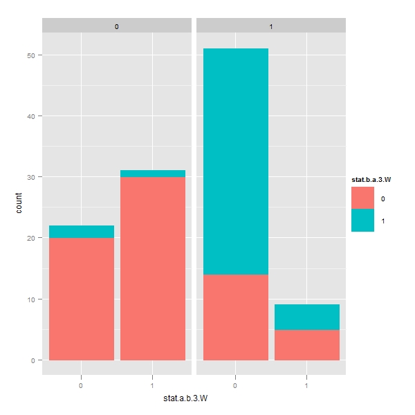
> p <- ggplot(temp, aes(x = stat.a.b.3.W, color = stat.b.a.3.W,
+     fill = stat.b.a.3.W))
> q <- p + geom_bar()
> print(q)
> q <- p + geom_bar() + facet_grid(. ~ stat.a.b.3)
> print(q)
> q <- p + geom_bar() + facet_grid(. ~ stat.b.a.3)
> print(q)

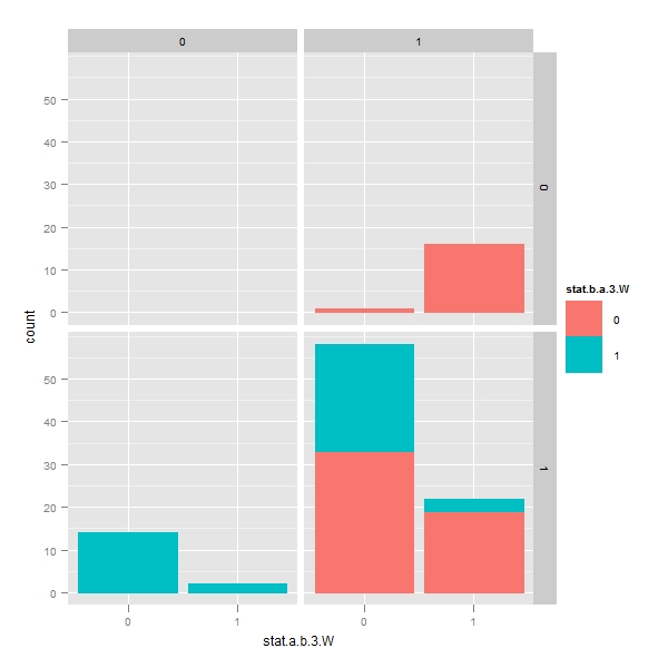
Faceting with chriss procedure

> q <- p + geom_bar() + facet_grid(stat.b.a.2 ~ stat.a.b.2)
> print(q)

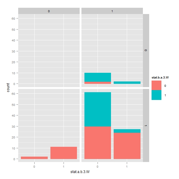
Faceting with lag term procedure

> q <- p + geom_bar() + facet_grid(stat.lag.a.b ~ stat.lag.b.a)
> print(q)

> p <- ggplot(temp, aes(x = stat.a.b.3, color = stat.b.a.3, fill = stat.b.a.3))
> q <- p + geom_bar()
> print(q)
> q <- p + geom_bar() + facet_grid(stat.lag.a.b ~ stat.lag.b.a)
> print(q)

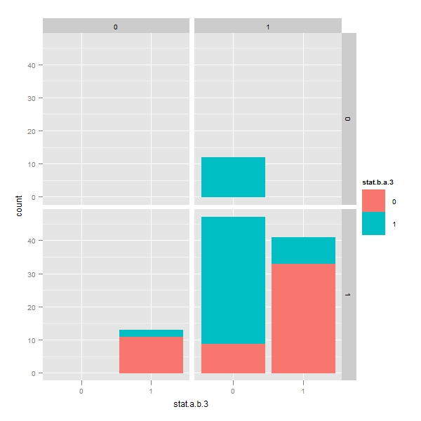
THE MOST IMPORTANT GRAPH OUT OF SPENDING ALMOST 6-7 HOURS !!! Faceting with pfaff procedure

> p <- ggplot(temp, aes(x = stat.a.b.3, color = stat.b.a.3, fill = stat.b.a.3))
> q <- p + geom_bar() + facet_grid(stat.b.a.3.W ~ stat.a.b.3.W)
> print(q)

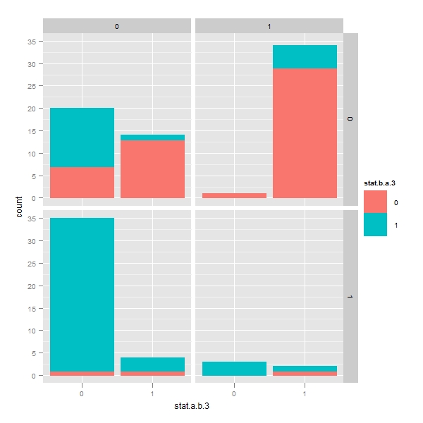
The above facet shows that in the second quadrant, there are about 35 pairs which do not show any granger causality. Out of which, 30 pairs pass the error correction mechanisms. These are out of the trading portfolio. I have to analyze these!

Why are 27 pairs which pass error correction model described by pfaff do not get picked up by Granger test ?

This is the question that needs to be answered..