Power of a test
Purpose
Power of a test
> mu <- 10 > sd <- 15 > n <- 50 > bands <- mu + c(-1, 1) * qnorm(0.975) * sd/sqrt(n) |
For a specific population with mu , sigma, n the confidence bands for mu are created Now, if the real mu were something else, let us plot the power of the null hypothesis mu = mu.new
> mu.new <- seq(0, 25, by = 1) > power.stat <- sapply(mu.new, function(x) (1 - abs(diff(pnorm(x - + bands)))) * 100) > plot(mu.new, power.stat, type = "l", col = "blue", lwd = 2) |
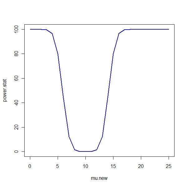
Take away - The farther the mean is , the more power the test is
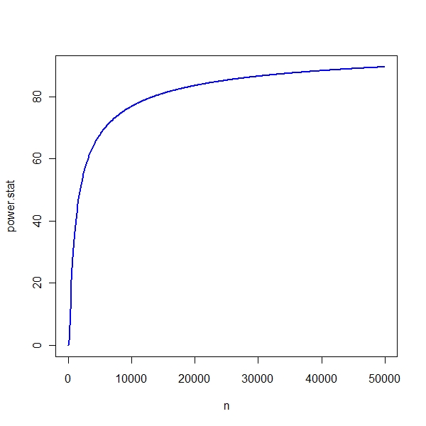
Now let us increase n and see how the power the test changes
> mu <- 10
> sd <- 15
> n <- seq(50, 50000, by = 100)
> bands <- matrix(data = NA, nrow = length(n), ncol = 2)
> for (i in seq_along(n)) bands[i, ] <- mu + c(-1, 1) * qnorm(0.975) *
+     sd/sqrt(n[i])
> mu.new <- 10
> power.stat <- matrix(data = NA, nrow = length(n), ncol = 1)
> for (i in seq_along(n)) {
+     temp <- ((1 - abs(diff(pnorm(mu.new - bands[i, ])))) * 100)
+     power.stat[i, ] <- temp
+ }
> plot(n, power.stat, type = "l", col = "blue", lwd = 2) |
Often in MBA or statistic text books, this aspect is brought out
and left at that stage.
However the key thing to note is that By increasing n, you are reducing the variance of the estimate and hence the power goes up.. Sometimes I think the only way that I can learn things is through simulation. Thanks R to giving me the insight in to power of a test.