John Fox Applied Reg - Chap 4
Purpose
DB - Fox - Regression. The usage of + - * / ^ in lm is going to be different. .Simulate a Multi reg ’’ .+
> n <- 1977
> set.seed(n)
> error.sd <- 3
> error <- sqrt(error.sd) * rnorm(n)
> true.beta <- rbind(2, 3, 4)
> indep <- cbind(rep(1, n), runif(n), runif(n))
> dep <- indep %*% true.beta + error
> fit <- lm(dep ~ indep[, 2] + indep[, 3])
> summary(fit)
Call:
lm(formula = dep ~ indep[, 2] + indep[, 3])

Residuals:
     Min       1Q   Median       3Q      Max
-5.69660 -1.10317  0.02548  1.11955  5.30918

Coefficients:
            Estimate Std. Error t value Pr(>|t|)
(Intercept)   1.9875     0.1014   19.60   <2e-16 ***
indep[, 2]    2.8206     0.1320   21.37   <2e-16 ***
indep[, 3]    4.1764     0.1340   31.18   <2e-16 ***
---
Signif. codes:  0 '***' 0.001 '**' 0.01 '*' 0.05 '.' 0.1 ' ' 1

Residual standard error: 1.709 on 1974 degrees of freedom
Multiple R-squared: 0.4195,     Adjusted R-squared: 0.4189
F-statistic: 713.2 on 2 and 1974 DF, p-value: < 2.2e-16 |
> n <- 1977
> set.seed(n)
> error.sd <- 3
> error <- sqrt(error.sd) * rnorm(n)
> true.beta <- rbind(2, 3, 4)
> indep <- cbind(rep(1, n), runif(n), runif(n))
> dep <- indep %*% true.beta + error
> fit <- lm(dep ~ indep[, 2] - indep[, 3])
> summary(fit)
Call:
lm(formula = dep ~ indep[, 2] - indep[, 3])

Residuals:
     Min       1Q   Median       3Q      Max
-7.19413 -1.43267 -0.07039  1.44780  6.05450

Coefficients:
            Estimate Std. Error t value Pr(>|t|)
(Intercept)  4.07416    0.09307   43.78   <2e-16 ***
indep[, 2]   2.81388    0.16121   17.45   <2e-16 ***
---
Signif. codes:  0 '***' 0.001 '**' 0.01 '*' 0.05 '.' 0.1 ' ' 1

Residual standard error: 2.087 on 1975 degrees of freedom
Multiple R-squared: 0.1336,     Adjusted R-squared: 0.1332
F-statistic: 304.7 on 1 and 1975 DF, p-value: < 2.2e-16 |
> n <- 1977
> set.seed(n)
> error.sd <- 3
> error <- sqrt(error.sd) * rnorm(n)
> true.beta <- rbind(2, 3, 4)
> indep <- cbind(rep(1, n), runif(n), runif(n))
> dep <- indep %*% true.beta + error
> fit <- lm(dep ~ indep[, 2] * indep[, 3])
> summary(fit)
Call:
lm(formula = dep ~ indep[, 2] * indep[, 3])

Residuals:
     Min       1Q   Median       3Q      Max
-5.69500 -1.10398  0.02508  1.12103  5.30697

Coefficients:
                      Estimate Std. Error t value Pr(>|t|)
(Intercept)            1.99090    0.15574  12.783   <2e-16 ***
indep[, 2]             2.81386    0.26792  10.502   <2e-16 ***
indep[, 3]             4.16967    0.26972  15.459   <2e-16 ***
indep[, 2]:indep[, 3]  0.01331    0.46198   0.029    0.977
---
Signif. codes:  0 '***' 0.001 '**' 0.01 '*' 0.05 '.' 0.1 ' ' 1

Residual standard error: 1.709 on 1973 degrees of freedom
Multiple R-squared: 0.4195,     Adjusted R-squared: 0.4186
F-statistic: 475.2 on 3 and 1973 DF, p-value: < 2.2e-16 |
/
> n <- 1977
> set.seed(n)
> error.sd <- 3
> error <- sqrt(error.sd) * rnorm(n)
> true.beta <- rbind(2, 3, 4)
> indep <- cbind(rep(1, n), runif(n), runif(n))
> dep <- indep %*% true.beta + error
> fit <- lm(dep ~ indep[, 2]/indep[, 3])
> summary(fit)
Call:
lm(formula = dep ~ indep[, 2]/indep[, 3])

Residuals:
     Min       1Q   Median       3Q      Max
-6.45644 -1.17190  0.04854  1.16028  5.65789

Coefficients:
                      Estimate Std. Error t value Pr(>|t|)
(Intercept)            4.09045    0.08069  50.694   <2e-16 ***
indep[, 2]            -0.31556    0.18579  -1.698   0.0896 .
indep[, 2]:indep[, 3]  6.21142    0.24296  25.566   <2e-16 ***
---
Signif. codes:  0 '***' 0.001 '**' 0.01 '*' 0.05 '.' 0.1 ' ' 1

Residual standard error: 1.81 on 1974 degrees of freedom
Multiple R-squared: 0.3491,     Adjusted R-squared: 0.3485
F-statistic: 529.5 on 2 and 1974 DF, p-value: < 2.2e-16 |
^
> n <- 1977
> set.seed(n)
> error.sd <- 3
> error <- sqrt(error.sd) * rnorm(n)
> true.beta <- rbind(2, 3, 4)
> indep <- cbind(rep(1, n), runif(n), runif(n))
> dep <- indep %*% true.beta + error
> fit <- lm(dep ~ I(indep[, 2]^2))
> summary(fit)
Call:
lm(formula = dep ~ I(indep[, 2]^2))

Residuals:
     Min       1Q   Median       3Q      Max
-7.07126 -1.46190 -0.08996  1.45188  6.24808

Coefficients:
                Estimate Std. Error t value Pr(>|t|)
(Intercept)      4.57679    0.07029   65.11   <2e-16 ***
I(indep[, 2]^2)  2.70063    0.15678   17.23   <2e-16 ***
---
Signif. codes:  0 '***' 0.001 '**' 0.01 '*' 0.05 '.' 0.1 ' ' 1

Residual standard error: 2.091 on 1975 degrees of freedom
Multiple R-squared: 0.1306,     Adjusted R-squared: 0.1302
F-statistic: 296.7 on 1 and 1975 DF,  p-value: < 2.2e-16
> fit <- lm(dep ~ (indep[, 2]^2))
> summary(fit)
Call:
lm(formula = dep ~ (indep[, 2]^2))

Residuals:
     Min       1Q   Median       3Q      Max
-7.19413 -1.43267 -0.07039  1.44780  6.05450

Coefficients:
            Estimate Std. Error t value Pr(>|t|)
(Intercept)  4.07416    0.09307   43.78   <2e-16 ***
indep[, 2]   2.81388    0.16121   17.45   <2e-16 ***
---
Signif. codes:  0 '***' 0.001 '**' 0.01 '*' 0.05 '.' 0.1 ' ' 1

Residual standard error: 2.087 on 1975 degrees of freedom
Multiple R-squared: 0.1336,     Adjusted R-squared: 0.1332
F-statistic: 304.7 on 1 and 1975 DF, p-value: < 2.2e-16 |
To remove a few observations from the old model
> n <- 1977
> set.seed(n)
> error.sd <- 3
> error <- sqrt(error.sd) * rnorm(n)
> true.beta <- rbind(2, 3, 4)
> indep <- cbind(rep(1, n), runif(n), runif(n))
> dep <- indep %*% true.beta + error
> fit <- lm(dep ~ indep[, 2] + indep[, 3])
> summary(fit)
Call:
lm(formula = dep ~ indep[, 2] + indep[, 3])

Residuals:
     Min       1Q   Median       3Q      Max
-5.69660 -1.10317  0.02548  1.11955  5.30918

Coefficients:
            Estimate Std. Error t value Pr(>|t|)
(Intercept)   1.9875     0.1014   19.60   <2e-16 ***
indep[, 2]    2.8206     0.1320   21.37   <2e-16 ***
indep[, 3]    4.1764     0.1340   31.18   <2e-16 ***
---
Signif. codes:  0 '***' 0.001 '**' 0.01 '*' 0.05 '.' 0.1 ' ' 1

Residual standard error: 1.709 on 1974 degrees of freedom
Multiple R-squared: 0.4195,     Adjusted R-squared: 0.4189
F-statistic: 713.2 on 2 and 1974 DF,  p-value: < 2.2e-16
> summary(update(fit, subset = -10))
Call:
lm(formula = dep ~ indep[, 2] + indep[, 3], subset = -10)

Residuals:
     Min       1Q   Median       3Q      Max
-5.69632 -1.10368  0.02294  1.12023  5.31033

Coefficients:
            Estimate Std. Error t value Pr(>|t|)
(Intercept)   1.9861     0.1015   19.57   <2e-16 ***
indep[, 2]    2.8219     0.1321   21.37   <2e-16 ***
indep[, 3]    4.1772     0.1340   31.17   <2e-16 ***
---
Signif. codes:  0 '***' 0.001 '**' 0.01 '*' 0.05 '.' 0.1 ' ' 1

Residual standard error: 1.709 on 1973 degrees of freedom
Multiple R-squared: 0.4194,     Adjusted R-squared: 0.4188
F-statistic: 712.7 on 2 and 1973 DF, p-value: < 2.2e-16 |
Want to do a standardized regression coeff
> z <- cbind(dep, indep)
> z <- scale(z)
> fit <- lm(z[, 1] ~ z[, 3] + z[, 4])
> summary(fit)
Call:
lm(formula = z[, 1] ~ z[, 3] + z[, 4])

Residuals:
     Min       1Q   Median       3Q      Max
-2.54100 -0.49208  0.01136  0.49938  2.36819

Coefficients:
             Estimate Std. Error  t value Pr(>|t|)
(Intercept) 9.868e-19  1.714e-02 5.76e-17        1
z[, 3]      3.664e-01  1.715e-02    21.37   <2e-16 ***
z[, 4]      5.346e-01  1.715e-02    31.18   <2e-16 ***
---
Signif. codes:  0 '***' 0.001 '**' 0.01 '*' 0.05 '.' 0.1 ' ' 1

Residual standard error: 0.7623 on 1974 degrees of freedom
Multiple R-squared: 0.4195,     Adjusted R-squared: 0.4189
F-statistic: 713.2 on 2 and 1974 DF, p-value: < 2.2e-16 |
Want to remove intercept from the model.
> z <- cbind(dep, indep)
> z <- scale(z)
> fit <- lm(z[, 1] ~ z[, 3] + z[, 4] - 1)
> summary(fit)
Call:
lm(formula = z[, 1] ~ z[, 3] + z[, 4] - 1)

Residuals:
     Min       1Q   Median       3Q      Max
-2.54100 -0.49208  0.01136  0.49938  2.36819

Coefficients:
       Estimate Std. Error t value Pr(>|t|)
z[, 3]  0.36644    0.01714   21.37   <2e-16 ***
z[, 4]  0.53463    0.01714   31.18   <2e-16 ***
---
Signif. codes:  0 '***' 0.001 '**' 0.01 '*' 0.05 '.' 0.1 ' ' 1

Residual standard error: 0.7621 on 1975 degrees of freedom
Multiple R-squared: 0.4195,     Adjusted R-squared: 0.4189
F-statistic: 713.5 on 2 and 1975 DF,  p-value: < 2.2e-16
> fit <- lm(z[, 1] ~ z[, 3] + z[, 4] + 0)
> summary(fit)
Call:
lm(formula = z[, 1] ~ z[, 3] + z[, 4] + 0)

Residuals:
     Min       1Q   Median       3Q      Max
-2.54100 -0.49208  0.01136  0.49938  2.36819

Coefficients:
       Estimate Std. Error t value Pr(>|t|)
z[, 3]  0.36644    0.01714   21.37   <2e-16 ***
z[, 4]  0.53463    0.01714   31.18   <2e-16 ***
---
Signif. codes:  0 '***' 0.001 '**' 0.01 '*' 0.05 '.' 0.1 ' ' 1

Residual standard error: 0.7621 on 1975 degrees of freedom
Multiple R-squared: 0.4195,     Adjusted R-squared: 0.4189
F-statistic: 713.5 on 2 and 1975 DF, p-value: < 2.2e-16 |
Change the dummy variable coding
> n <- 2000 > set.seed(n) > error.sd <- 3 > error <- sqrt(error.sd) * rnorm(n) > true.beta <- rbind(2, 3, 4) > indep <- cbind(rep(1, n), runif(n), runif(n)) > dep <- indep %*% true.beta + error > z <- as.data.frame(cbind(dep, indep)) > z$fac <- factor(rep(letters[1:4], 500)) > contrasts(z$fac) b c d a 0 0 0 b 1 0 0 c 0 1 0 d 0 0 1 |
Change the base coding to
> contrasts(z$fac) <- contr.treatment(levels(z$fac), base = 2) > contrasts(z$fac) a c d a 1 0 0 b 0 0 0 c 0 1 0 d 0 0 1 |
Run a reg with factor a as base
> n <- 2000
> set.seed(n)
> error.sd <- 3
> error <- sqrt(error.sd) * rnorm(n)
> true.beta <- rbind(2, 3, 4)
> indep <- cbind(rep(1, n), runif(n), runif(n))
> dep <- indep %*% true.beta + error
> z <- as.data.frame(cbind(dep, indep))
> z$fac <- factor(rep(letters[1:4], 500))
> fit <- lm(z[, 1] ~ z[, 3] + z[, 4] + z$fac)
> summary(fit)
Call:
lm(formula = z[, 1] ~ z[, 3] + z[, 4] + z$fac)

Residuals:
     Min       1Q   Median       3Q      Max
-5.75244 -1.15317 -0.03433  1.18877  5.13664

Coefficients:
            Estimate Std. Error t value Pr(>|t|)
(Intercept)  2.14092    0.11970  17.886   <2e-16 ***
z[, 3]       2.99510    0.13357  22.423   <2e-16 ***
z[, 4]       3.87625    0.13317  29.107   <2e-16 ***
z$facb      -0.03152    0.10841  -0.291    0.771
z$facc      -0.01576    0.10838  -0.145    0.884
z$facd      -0.09286    0.10838  -0.857    0.392
---
Signif. codes:  0 '***' 0.001 '**' 0.01 '*' 0.05 '.' 0.1 ' ' 1

Residual standard error: 1.713 on 1994 degrees of freedom
Multiple R-squared: 0.4063,     Adjusted R-squared: 0.4048
F-statistic: 272.9 on 5 and 1994 DF, p-value: < 2.2e-16 |
Run a reg with factor b as base
> n <- 2000
> set.seed(n)
> error.sd <- 3
> error <- sqrt(error.sd) * rnorm(n)
> true.beta <- rbind(2, 3, 4)
> indep <- cbind(rep(1, n), runif(n), runif(n))
> dep <- indep %*% true.beta + error
> z <- as.data.frame(cbind(dep, indep))
> z$fac <- factor(rep(letters[1:4], 500))
> contrasts(z$fac) <- contr.treatment(levels(z$fac), base = 2)
> fit <- lm(z[, 1] ~ z[, 3] + z[, 4] + z$fac)
> summary(fit)
Call:
lm(formula = z[, 1] ~ z[, 3] + z[, 4] + z$fac)

Residuals:
     Min       1Q   Median       3Q      Max
-5.75244 -1.15317 -0.03433  1.18877  5.13664

Coefficients:
            Estimate Std. Error t value Pr(>|t|)
(Intercept)  2.10940    0.12157  17.351   <2e-16 ***
z[, 3]       2.99510    0.13357  22.423   <2e-16 ***
z[, 4]       3.87625    0.13317  29.107   <2e-16 ***
z$faca       0.03152    0.10841   0.291    0.771
z$facc       0.01576    0.10840   0.145    0.884
z$facd      -0.06135    0.10838  -0.566    0.571
---
Signif. codes:  0 '***' 0.001 '**' 0.01 '*' 0.05 '.' 0.1 ' ' 1

Residual standard error: 1.713 on 1994 degrees of freedom
Multiple R-squared: 0.4063,     Adjusted R-squared: 0.4048
F-statistic: 272.9 on 5 and 1994 DF, p-value: < 2.2e-16 |
See the anova of the model
> anova(fit)
Analysis of Variance Table

Response: z[, 1]
            Df Sum Sq Mean Sq  F value Pr(>F)
z[, 3]       1 1516.2  1516.2 516.4704 <2e-16 ***
z[, 4]       1 2487.2  2487.2 847.2168 <2e-16 ***
z$fac        3    2.5     0.8   0.2813  0.839
Residuals 1994 5853.8     2.9
---
Signif. codes: 0 '***' 0.001 '**' 0.01 '*' 0.05 '.' 0.1 ' ' 1 |
- Best thing is to test the goodness of fit relating to two models
> fit1 <- lm(z[, 1] ~ z[, 3] + z[, 4]) > fit2 <- lm(z[, 1] ~ z[, 3] + z[, 4] + z$fac) > anova(fit1, fit2) Analysis of Variance Table Model 1: z[, 1] ~ z[, 3] + z[, 4] Model 2: z[, 1] ~ z[, 3] + z[, 4] + z$fac Res.Df RSS Df Sum of Sq F Pr(>F) 1 1997 5856.3 2 1994 5853.8 3 2.5 0.2813 0.839 |
Basic Hypo testing
> library(car)
> attach(Duncan)
The following object(s) are masked from Duncan ( position 3 ) :
education income prestige type
|
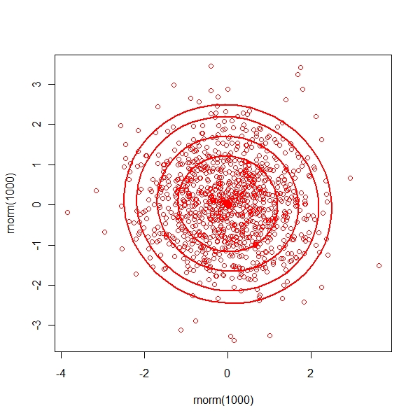
Check for elliptical plots between two normal distributions
> data.ellipse(rnorm(1000), rnorm(1000), levels = c(0.5, 0.75, + 0.9, 0.95)) |
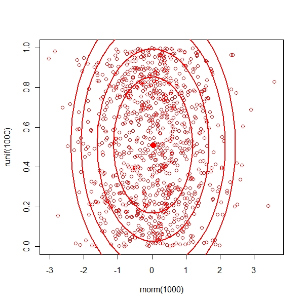
Check for elliptical plots between a normal and a uniform distributions
> data.ellipse(rnorm(1000), runif(1000), levels = c(0.5, 0.75, + 0.9, 0.95)) |
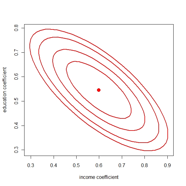
Confidence plots for estimates
> fit <- lm(prestige ~ income + education) > confidence.ellipse(fit, levels = c(0.5, 0.75, 0.9, 0.95)) |
Arguments for lm
> args(lm)
function (formula, data, subset, weights, na.action, method = "qr",
    model = TRUE, x = FALSE, y = FALSE, qr = TRUE, singular.ok = TRUE,
    contrasts = NULL, offset, ...)
NULL |
Use of Identity
> fit <- lm(prestige ~ I(income + education))
> summary(fit)
Call:
lm(formula = prestige ~ I(income + education))

Residuals:
     Min       1Q   Median       3Q      Max
-29.6049  -6.7078   0.1235   6.9794  33.2895

Coefficients:
                      Estimate Std. Error t value Pr(>|t|)
(Intercept)           -6.06319    4.22540  -1.435    0.159
I(income + education)  0.56927    0.03958  14.382   <2e-16 ***
---
Signif. codes:  0 '***' 0.001 '**' 0.01 '*' 0.05 '.' 0.1 ' ' 1

Residual standard error: 13.22 on 43 degrees of freedom
Multiple R-squared: 0.8279,     Adjusted R-squared: 0.8239
F-statistic: 206.8 on 1 and 43 DF,  p-value: < 2.2e-16
> fit <- lm(prestige ~ I(income * education))
> summary(fit)
Call:
lm(formula = prestige ~ I(income * education))

Residuals:
    Min      1Q  Median      3Q     Max
-30.559 -10.845  -1.661   5.826  49.967

Coefficients:
                       Estimate Std. Error t value Pr(>|t|)
(Intercept)           1.728e+01  3.425e+00   5.044 8.75e-06 ***
I(income * education) 1.120e-02  9.385e-04  11.934 3.10e-15 ***
---
Signif. codes:  0 '***' 0.001 '**' 0.01 '*' 0.05 '.' 0.1 ' ' 1

Residual standard error: 15.35 on 43 degrees of freedom
Multiple R-squared: 0.7681,     Adjusted R-squared: 0.7627
F-statistic: 142.4 on 1 and 43 DF,  p-value: 3.102e-15
> fit <- lm(prestige ~ (income * education))
> summary(fit)
Call:
lm(formula = prestige ~ (income * education))

Residuals:
     Min       1Q   Median       3Q      Max
-29.1898  -6.2758   0.4532   7.0933  32.7585

Coefficients:
                  Estimate Std. Error t value Pr(>|t|)
(Intercept)      -8.250934   7.378546  -1.118  0.26998
income            0.655621   0.197148   3.326  0.00187 **
education         0.606030   0.192363   3.150  0.00304 **
income:education -0.001237   0.003386  -0.365  0.71673
---
Signif. codes:  0 '***' 0.001 '**' 0.01 '*' 0.05 '.' 0.1 ' ' 1

Residual standard error: 13.51 on 41 degrees of freedom
Multiple R-squared: 0.8287,     Adjusted R-squared: 0.8162
F-statistic: 66.13 on 3 and 41 DF,  p-value: 9.286e-16
> fit <- lm(prestige ~ (income:education))
> summary(fit)
Call:
lm(formula = prestige ~ (income:education))

Residuals:
    Min      1Q  Median      3Q     Max
-30.559 -10.845  -1.661   5.826  49.967

Coefficients:
                  Estimate Std. Error t value Pr(>|t|)
(Intercept)      1.728e+01  3.425e+00   5.044 8.75e-06 ***
income:education 1.120e-02  9.385e-04  11.934 3.10e-15 ***
---
Signif. codes:  0 '***' 0.001 '**' 0.01 '*' 0.05 '.' 0.1 ' ' 1

Residual standard error: 15.35 on 43 degrees of freedom
Multiple R-squared: 0.7681,     Adjusted R-squared: 0.7627
F-statistic: 142.4 on 1 and 43 DF, p-value: 3.102e-15 |