Dobson - GLM - Chap 2 -Exercises

Purpose
Work out the chapter 2 exercises from dobson book on Generalized Linear models

Problem 1

> x <- read.csv("test4.csv", header = T, stringsAsFactors = T)
> head(x)
  test control
1 4.81    4.17
2 4.17    3.05
3 4.41    5.18
4 3.59    4.01
5 5.87    6.11
6 3.83    4.10

a)Summary

> summary(x)
      test          control
 Min.   :3.480   Min.   :3.050
 1st Qu.:4.388   1st Qu.:4.077
 Median :4.850   Median :4.635
 Mean   :4.860   Mean   :4.726
 3rd Qu.:5.390   3rd Qu.:5.393
 Max.   :6.340   Max.   :6.110

Boxplot of test and control

> boxplot(x)

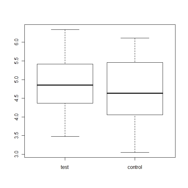
Control is showing a slightly more deviation

> stem(x[, 1])
  The decimal point is at the |

  3 | 568
  4 | 234477899
  5 | 024589
  6 | 03
> stem(x[, 2])
  The decimal point is at the |

  3 | 0679
  4 | 0125567
  5 | 1223666
  6 | 01

Looks like left skewed

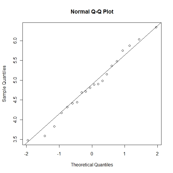
Test Quantile Plot

> qqnorm(x[, 1])
> qqline(x[, 1])

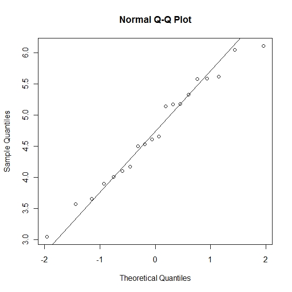
Control Quantile Plot

> qqnorm(x[, 2])
> qqline(x[, 2])

b)Unpaired t test

> t.test(x[, 1], x[, 2])
        Welch Two Sample t-test

data:  x[, 1] and x[, 2]
t = 0.5098, df = 37.711, p-value = 0.6131
alternative hypothesis: true difference in means is not equal to 0
95 percent confidence interval:
 -0.3967069  0.6637069
sample estimates:
mean of x mean of y
   4.8600    4.7265

No difference in means

c) test the model

> y <- c(x[, 1], x[, 2])
> SS0 <- sum((y - mean(y))^2)
> SS1 <- sum((x[, 1] - mean(x[, 1]))^2) + sum((x[, 2] - mean(x[,
+     2]))^2)
> Fstat <- (SS0 - SS1)/(SS1/38)
> sqrt(Fstat)
[1] 0.5098476
> qf(Fstat, 1, 38)
[1] 0.1116992

As you can see that sqrt of Fstat is tstat
and from the F test you reject the alternate.

Problem 2

> x <- read.csv("test5.csv", header = T, stringsAsFactors = T)
> head(x)
  man before after
1   1  100.8  97.0
2   2  102.0 107.5
3   3  105.9  97.0
4   4  108.0 108.0
5   5   92.0  84.0
6   6  116.7 111.5
> t.test(x$before, x$after)
        Welch Two Sample t-test

data:  x$before and x$after
t = 0.6431, df = 37.758, p-value = 0.5241
alternative hypothesis: true difference in means is not equal to 0
95 percent confidence interval:
 -5.683035 10.973035
sample estimates:
mean of x mean of y
  103.245   100.600
> t.test(x$before - x$after)
        One Sample t-test

data:  x$before - x$after
t = 2.8734, df = 19, p-value = 0.00973
alternative hypothesis: true mean is not equal to 0
95 percent confidence interval:
 0.718348 4.571652
sample estimates:
mean of x
    2.645

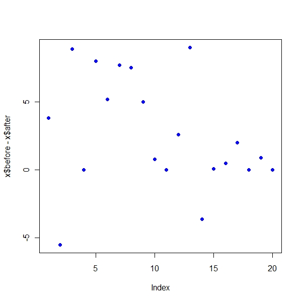
As you can see that unpaired test says that there is no difference between means WHILE pairs test clearly shows that there is a difference inmeans

> plot(x$before - x$after, pch = 19, col = "blue")