Chap 4 - Exercise 4.1

> setwd("C:/Cauldron/garage/R/soulcraft/Volatility/Learn/Dobson-GLM")
> data <- read.csv("test8.csv", header = T, stringsAsFactors = F)
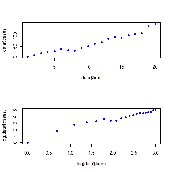
> par(mfrow = c(2, 1))
> plot(data$time, data$cases, pch = 19, col = "blue", cex = 1)
> plot(log(data$time), log(data$cases), pch = 19, col = "blue",
+     cex = 1)

> beta0 <- c(3, 1)
> n <- dim(data)[1]
> data$logt <- log(data$time)
> poisreg <- function(beta0) {
+     beta <- matrix(data = beta0, ncol = 1)
+     X <- cbind(rep(1, n), data$logt)
+     W <- diag(n)
+     diag(W) <- exp(X %*% beta)
+     LHS <- t(X) %*% W %*% X
+     z <- matrix(data = NA, nrow = n, ncol = 1)
+     z <- X %*% beta0 + (data$cases - exp(X %*% beta))/exp(X %*%
+         beta)
+     RHS <- t(X) %*% W %*% z
+     beta.res <- solve(LHS, RHS)
+     return(beta.res)
+ }
> iterations <- matrix(data = NA, nrow = 2, ncol = 150)
> iterations[, 1] <- poisreg(beta0)
> for (i in 2:150) {
+     iterations[, (i)] <- poisreg(iterations[, (i - 1)])
+ }
> print(iterations[, 150])
[1] 0.995998 1.326610

> W <- diag(n)
> diag(W) <- exp(X %*% iterations[, 150])
> X <- cbind(rep(1, n), data$logt)
> J <- t(X) %*% W %*% X
> Jinv <- solve(J)

> iterations[, 150]
[1] 0.995998 1.326610
> iterations[1, 150] + sqrt(Jinv[1, 1]) * 1.96 * c(-1, 1)
[1] 0.6633711 1.3286250
> iterations[2, 150] + sqrt(Jinv[2, 2]) * 1.96 * c(-1, 1)
[1] 1.199928 1.453292

> model.pois <- glm(data$cases ~ data$logt, family = poisson(link = log))
> summary(model.pois)
Call:
glm(formula = data$cases ~ data$logt, family = poisson(link = log))

Deviance Residuals:
    Min       1Q   Median       3Q      Max
-2.0568  -0.8302  -0.3072   0.9279   1.7310

Coefficients:
            Estimate Std. Error z value Pr(>|z|)
(Intercept)  0.99600    0.16971   5.869 4.39e-09 ***
data$logt    1.32661    0.06463  20.525  < 2e-16 ***
---
Signif. codes:  0 '***' 0.001 '**' 0.01 '*' 0.05 '.' 0.1 ' ' 1

(Dispersion parameter for poisson family taken to be 1)

    Null deviance: 677.264  on 19  degrees of freedom
Residual deviance:  21.755  on 18  degrees of freedom
AIC: 138.05

Number of Fisher Scoring iterations: 4