Attilio Meucci - Chapter 1
Purpose
Playground for Chapter 1 - Risk and Asset Allocation - Attilio Meucci
- Basic moments of UNIF
> n <- 10000 > x <- runif(n) > location <- mean(x) > dispersion <- sd(x) > skewness <- sum((x - 0.5)^3)/(n * (sd(x))^3) > kurtosis <- sum((x - 0.5)^4)/(n * (sd(x))^4) > print(paste(location, dispersion, skewness, kurtosis, sep = " ")) [1] "0.500898264411953 0.289608228592819 0.00694912472323462 1.80087482669602" |
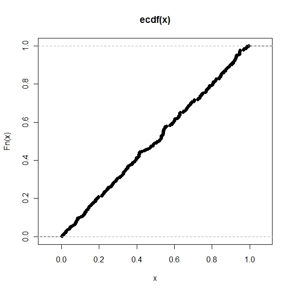
- ecdf for unif
> par(mfrow = c(1, 1)) > x <- runif(300) > plot(ecdf(x)) |
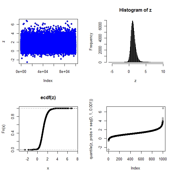
- T and Normal
> df <- 8 > mu1 <- 0 > var1 <- 0.1 > n <- 1e+05 > x <- mu1 + sqrt(var1) * rt(n, df = df) > mu2 <- 0.1 > var2 <- 0.2 > y <- rlnorm(n, meanlog = mu2, sdlog = sqrt(var2)) > z <- x + y |
> par(mfrow = c(2, 2)) > plot(z, pch = 19, col = "blue") > hist(z, breaks = c(seq(-6, 10, 0.1))) > z1 <- ecdf(z) > plot(z1) > plot(quantile(z, probs = seq(0, 1, 0.001))) |
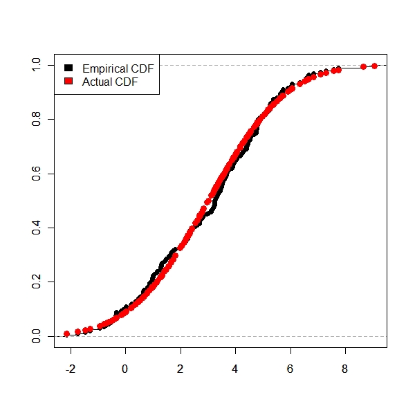
- Empirical CDF and Actual CDF
> par(mfrow = c(1, 1))
> n <- 200
> x <- rnorm(n, 3, sqrt(5))
> y <- x[order(x, decreasing = F)]
> plot(ecdf(y), ylim = c(0, 1), xlim = range(y), xlab = "", ylab = "",
+     main = "")
> actual.cdf <- pnorm(y, 3, sqrt(5))
> par(new = T)
> plot(y, actual.cdf, col = "red", pch = 19, cex = 1.2, xlim = range(y),
+     ylim = c(0, 1), xlab = "", ylab = "", main = "")
> legend("topleft", legend = c("Empirical CDF", "Actual CDF"),
+ fill = c("black", "red")) |
1.2.2. Generalized T
> var1 <- 6
> mu1 <- 2
> n <- 1e+05
> iterations <- 20
> results <- matrix(data = NA, nrow = iterations, ncol = 2)
> for (df in 1:iterations) {
+     x <- mu1 + sqrt(var1) * rt(n, df = df)
+     results[df, 1] <- abs(var(x) - 7)
+     results[df, 2] <- df
+ }
> results[which(results[, 1] == min(results[, 1])), ]
[1]  0.0269576 14.0000000
> 2/(1 - 6/7)
[1] 14 |
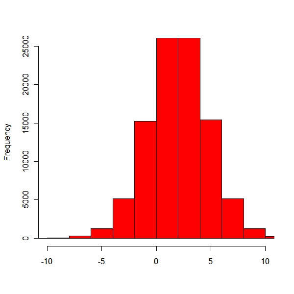
Student t
> x.old <- mu1 + sqrt(var1) * rt(n, df = 14) > y <- rnorm(n, 0, sqrt(var1)) > z <- rchisq(n, 14) > x.new <- mu1 + y/sqrt(z/15) > par(mfrow = c(1, 1)) > hist(x.old, xlim = c(-10, 10), col = "blue", ylim = c(0, 25000), + main = "", xlab = "") > par(new = T) > hist(x.new, xlim = c(-10, 10), col = "red", ylim = c(0, 25000), + main = "", xlab = "") |
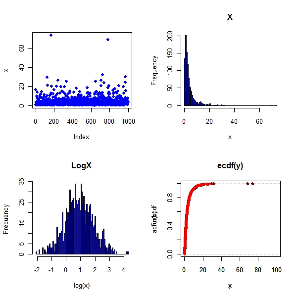
LogNormal Distribution
> mu.x <- 3 > var.x <- 5 > n <- 1000 > var.u <- log(1 + var.x/mu.x) > mu.u <- log(mu.x) - 0.5 * log(1 + var.x/(mu.x * mu.x)) > x <- rlnorm(n, meanlog = mu.u, sdlog = sqrt(var.u)) > y <- x[order(x, decreasing = F)] > actual.cdf <- plnorm(y, meanlog = mu.u, sdlog = sqrt(var.u)) > par(mfrow = c(2, 2)) > plot(x, pch = 19, col = "blue") > hist(x, col = "blue", main = "X", breaks = c(seq(min(x), max(x), + length = 100))) > hist(log(x), col = "blue", main = "LogX", breaks = c(seq(min(log(x)), + max(log(x)), length = 100))) > plot(ecdf(y), xlim = c(0, 100)) > par(new = T) > plot(y, actual.cdf, xlim = c(0, 100), col = "red") |
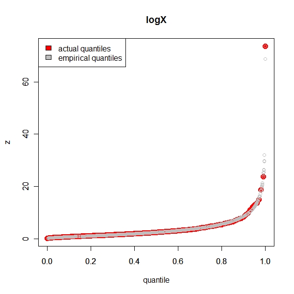
Empirical Quantile Vs Exact Quantile
> par(mfrow = c(1, 1))
> z <- data.frame(quantiles = (quantile(y, prob = seq(0, 1, 0.01))))
> z$qts <- seq(0, 1, 0.01)
> plot(z$qts, z[, 1], pch = 19, col = "red", xlab = "quantile",
+     ylab = "z", xlim = c(0, 1), cex = 1.5, main = "logX")
> par(new = T)
> plot(actual.cdf, y, xlim = c(0, 1), col = "grey", xlab = "",
+     ylab = "")
> legend("topleft", legend = c("actual quantiles", "empirical quantiles"),
+ fill = c("red", "grey")) |
Gamma Vs Chi Square
> n <- 10000
> mu <- 0
> sig <- 1
> z1 <- matrix(data = NA, nrow = n, ncol = 11)
> for (i in 1:10) {
+     z1[, i] <- (rnorm(n, mu, sig))^2
+ }
> z1[, 11] <- rowSums(z1[, 1:10])
> rad <- z1[order(z1[, 11], decreasing = F), 11]
> par(mfrow = c(1, 1))
> actual.cdf <- pchisq(rad, 10)
> plot(ecdf(rad), xlim = c(0, 30), main = " Gamma Vs Chi Square",
+     xlab = "", ylab = "")
> par(new = T)
> plot(rad, actual.cdf, xlim = c(0, 30), col = "red", cex = 0.3,
+     xlab = "", ylab = "", main = "")
> legend("topleft", legend = c("chi sq cdf", "empirical gamma cdf"),
+ fill = c("red", "black")) |