Heteroskedasticity Tests

> set.seed(1977)
> n <- 1500
> beta.actual <- matrix(c(2, 3), ncol = 1)
> beta.sample <- cbind(rnorm(n, beta.actual[1]), rnorm(n, beta.actual[2]))
> error <- c(rnorm(n/2), rnorm(n/2, 0, 3))
> x <- cbind(rep(1, n), seq(from = 1, to = 5, length.out = n))
> y <- x[, 1] * beta.sample[, 1] + x[, 2] * beta.sample[, 2] +
+     error
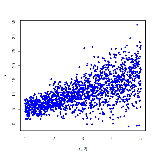
> plot(x[, 2], y, pch = 19, col = "blue")
> summary(lm(y ~ x + 0))
Call:
lm(formula = y ~ x + 0)

Residuals:
      Min        1Q    Median        3Q       Max
-17.01448  -2.13231   0.07604   2.19407  17.87364

Coefficients:
   Estimate Std. Error t value Pr(>|t|)
x1  2.08587    0.28936   7.209 8.93e-13 ***
x2  2.91157    0.09001  32.348  < 2e-16 ***
---
Signif. codes:  0 '***' 0.001 '**' 0.01 '*' 0.05 '.' 0.1 ' ' 1

Residual standard error: 4.028 on 1498 degrees of freedom
Multiple R-squared: 0.888,      Adjusted R-squared: 0.8878
F-statistic:  5936 on 2 and 1498 DF,  p-value: < 2.2e-16
> coef(lm(y ~ x + 0))
      x1       x2
2.085867 2.911567

> gqtest(y ~ x[, 2])
        Goldfeld-Quandt test

data:  y ~ x[, 2]
GQ = 4.3728, df1 = 748, df2 = 748, p-value < 2.2e-16

> x.t <- rep(c(-1, 1), 50)
> err1 <- rnorm(100, sd = rep(c(1, 2), 50))
> err2 <- rnorm(100)
> y1 <- 1 + x.t + err1
> y2 <- 1 + x.t + err2
> bptest(y1 ~ x.t)
        studentized Breusch-Pagan test

data:  y1 ~ x.t
BP = 12.1028, df = 1, p-value = 0.0005035
> bptest(y2 ~ x.t)
        studentized Breusch-Pagan test

data:  y2 ~ x.t
BP = 1.2061, df = 1, p-value = 0.2721

> library(lmtest)
> bptest(y ~ x[, 2] + I(x[, 2]^2) + 0)
        studentized Breusch-Pagan test

data:  y ~ x[, 2] + I(x[, 2]^2) + 0
BP = 176.1623, df = 1, p-value < 2.2e-16

> library(fArma)
> n <- 1500
> beta.actual <- matrix(c(2, 3), ncol = 1)
> beta.sample <- cbind(rnorm(n, beta.actual[1]), rnorm(n, beta.actual[2]))
> error <- c(rnorm(n/2), rnorm(n/2, 0, 3))
> x <- cbind(rep(1, n), seq(from = 1, to = 5, length.out = n))
> er.ar <- arima.sim(list(order = c(1, 0, 0), ar = c(0.9)), n = n)
> y <- x[, 1] * beta.sample[, 1] + x[, 2] * beta.sample[, 2] +
+     er.ar
> plot(x[, 2], y, pch = 19, col = "blue")
> summary(lm(y ~ x + 0))
Call:
lm(formula = y ~ x + 0)

Residuals:
      Min        1Q    Median        3Q       Max
-14.82168  -2.49701   0.02933   2.46448  13.68807

Coefficients:
   Estimate Std. Error t value Pr(>|t|)
x1  2.15368    0.28692   7.506 1.04e-13 ***
x2  3.04792    0.08925  34.151  < 2e-16 ***
---
Signif. codes:  0 '***' 0.001 '**' 0.01 '*' 0.05 '.' 0.1 ' ' 1

Residual standard error: 3.994 on 1498 degrees of freedom
Multiple R-squared: 0.8979,     Adjusted R-squared: 0.8977
F-statistic:  6584 on 2 and 1498 DF,  p-value: < 2.2e-16
> dwtest(y ~ x + 0)
        Durbin-Watson test

data:  y ~ x + 0
DW = 1.4457, p-value < 2.2e-16
alternative hypothesis: true autocorrelation is greater than 0

> cochrane.orcutt.lm <- function(mod) {
+     X <- model.matrix(mod)
+     y <- model.response(model.frame(mod))
+     e <- residuals(mod)
+     n <- length(e)
+     names <- colnames(X)
+     rho <- sum(e[1:(n - 1)] * e[2:n])/sum(e^2)
+     y <- y[2:n] - rho * y[1:(n - 1)]
+     X <- X[2:n, ] - rho * X[1:(n - 1), ]
+     mod <- lm(y ~ X - 1)
+     result <- list()
+     result$coefficients <- coef(mod)
+     names(result$coefficients) <- names
+     summary <- summary(mod, corr = F)
+     result$cov <- (summary$sigma^2) * summary$cov.unscaled
+     dimnames(result$cov) <- list(names, names)
+     result$sigma <- summary$sigma
+     result$rho <- rho
+     class(result) <- "cochrane.orcutt"
+     result
+ }
> cochrane.orcutt.lm(lm(y ~ x[, 2]))
$coefficients
(Intercept)      x[, 2]
   2.132841    3.053598

$cov
            (Intercept)      x[, 2]
(Intercept)  0.14579406 -0.04230266
x[, 2]      -0.04230266  0.01408982

$sigma
[1] 3.837711

$rho
[1] 0.276815

attr(,"class")
[1] "cochrane.orcutt"