A Primer for Unit Root Testing : Summary

There are two issues which have been occupying my mind ever since the trades that I had suggested have gone wrong.

1. Type I error( trade when there is no signal) , i.e trade when the series is non stationary. Typically this is relevant to unit root testing where the null hypothesis says the series is random.

2. Is the spread  really a result of cointegrated time series ?

   Each issue requires detailed understanding of time series concepts. This post deals with the first aspect.

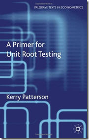
Unit root testing is one of the most involved areas of econometric analysis. This test requires a working knowledge of probability distributions , stochastic calculus, matrix algebra , Monte carlo simulation techniques to name a few. Needless to say , there are a lot of techniques for unit root testing and the literature is extensive. However the literature is sharply divided in 2 categories. The first category comprises explanations which are intuitive and that is all there is to it. You can probably explain and verbalize the intuition behind it but as a practitioner you would have difficulty in actually testing/ carrying out unit root tests.  The second category comprises dense econometric literature where there is extensive use of stochastic calculus, measure theory and simulations. So, there is an obvious need to bridge this gap in the literature and the book , “A Primer for Unit Root Testing”, serves exactly this purpose

This is probably the first time that I am writing about a book which is not even released . Amazon Store says that the book is slated to be released on April 27th 2010. The book is insanely priced at $110 , a tag which is too high for a book which claims to be a primer!. Anyways , the book is available as a torrent obviously at $0 :)

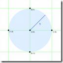
There can be no long-short trade if you are not reasonably certain that spread is a sample realization of a stationary process. So, in that sense, stationarity property is crucial for statistical arbitrage trading. In stats jargon you need to be sure that the series does not have a unit root. Actually the terminology arises from the fact that the roots of the characteristic equation should lie outside  a unit circle and hence the name called the unit root, Alternatively, the eigen vectors associated should all lie with in a unit circle.

This book is titled Primer to Unit root testing and the core of unit root is actually covered in the last chapter of the book. There are about 8 chapters in the book and the last chapter is on unit root tests! Then what is contained in the first  7 chapters. All these chapters deal with the principles that would be needed to do a basic unit root test.  Well to do an unit root test, it is easy to run a command in R/Matlab . But if you want to understand the nuts and bolts of various unit root tests and structural tests, a solid understanding of stochastic processes is a must and here is where the book fills the need. For those who have gone through Shreve, the first 7 chapters will serve a quick recap/ reminder of stuff that is present in Shreve.

Chapter – 1 :Introduction to Probability and Random Variables

The first chapter , “Introduction to Probability and Random Variables” , provides a basic introduction to measure theory, probability spaces, random variables, stationary processes etc. These are the basic principles based on which stationarity conditions can be tested. 

Often the math behind the symbols Ω, F , Ρ , Β in many books is explained in such a detailed manner with symbols, theorems, proofs etc that the basic intuition behind these symbols is lost. Pick any book on probability, the measure theoretic introduction is so abstract that it requires tremendous amount of motivation to get through the initial stuff. This chapter gives an intuitive feel of Sample space, Sigma fields, Borel Sets, Borel functions, Probability functions etc. The important point of defining probability measure for a Borel set and Borel field in R is intuitively explained by the issue that it is painful to define probabilities for points. Probability measures are assigned to Borel sets in R and hence there should be tools to define and manipulate these measures. These tools are nothing but the cumulative density function and density functions with respect to the random variable.

The connection between (sample space Ω, F sigma field of an Algebra, P probability measure) and (Real Space , Borel sets) in the real space is necessary to understand the basic principles of stochastic process. One must intuitively understand the connection between (Ω, ƒ , Ρ) ↔ (R,Β) and then know the math behind it. Often times, especially students who learn this in a formal course at a university, find that the equation is reversed. They will know the definitions and proofs of things relating to these but do not intuitively understand the stuff. Obviously, they will never be able to apply to practical problems.

There is also a mention of basic definitions of conditional probability, function of random variable, independence of random variables, expectations, covariance structure, correlations, Basic laws of expectations relating to random variables etc

A mention of law of iterated expectations in this chapter is made, intention being that it will be useful in understanding calculations relating to stochastic processes and unit root testing. What is law of iterated expectation? Taleb puts it in a nice way, in his book, “Blackswan”

If you expect that you will know tomorrow with certainty that your boyfriend has been cheating on you all this time, then you know today with certainty that your boyfriend is cheating on you and will take action today, say, by grabbing a pair of scissors and angrily cutting all his Ferragamo ties in half. You won’t tell yourself, This is what I will figure out tomorrow, but today is different so I will ignore the information and have a pleasant dinner. This point can be generalized to all forms of knowledge. There is actually a law in statistics called the law of iterated expectations, which I outline here in its strong form: if I expect to expect something at some date in the future, then I already expect that something at present.

The chapter then introduces stationarity. Strong stationarity arises when the joint distribution of the random variables is time invariant. This is far more difficult to test than weak form. Weak Stationarity arises when the stochastic process has a constant mean, constant variance and a covariance structure that is time invariant. Usually strong stationarity means weak stationarity but it is not always the case. There are examples where one cannot calculate moments and hence a series which is strongly stationary need not be weakly stationary. Partial sums of variables also give rise to weak stationary series which are extensively used in unit root testing.

Prima facie, the importance of stationarity lies in the fact that process parameters can be estimated by choosing any sample portion of the series. It does not matter which sample portion of the data is used for parameter estimation. One important aspect to be kept in mind is that, stationarity refers to a property of the process generating the outcomes. So, one must use the terms stationary process or non stationary process instead of stationary data / non stationary data. The word stationary data has no meaning. Stationarity is a property of the process. But I guess it is ok to use the words in whatever manner one wants to, as long as the intent is clearly communicated.

Chapter – 2 :Time Series

This chapter is a very basic intro to time series through lag operators. The usage of lag operators in simplifying calculations relating to arma processes are shown. White Noise, IIDs, Normal IIDs , Martingale Difference Sequences are mentioned as these form the components of ARMA processes, based on the kind of model that one is dealing with. Most of anti-quant group might object saying, “How the hell do you know that error terms follow some DGP( Data generative process) ? “ for which nobody has an answer. In any case if you want to do something with the data, than just be in the zen state , there one can use time series fundas and atleast try to get some hang of the data patterns. Whenever someone asks this question, my only answer would be “ there is no harm in modeling when you are dealing or living in the HIGH FREQ WORLD“. 

Invertibility is discussed in the context of computational necessity for estimating the parameters. Measure of persistence is defined and the first glimpse of the ways to measure non stationarity is provided. AR polynomial equation which has a unit root or roots with in a unit circle behaves in such a way that measure of persistence does not converge and increases with out limit. A whole lot of ARMA estimation procedures are covered at a 10,000 ft level often referring to the estimation, inference of parameters to some software results. One of the takeaways from this chapter is the concept of long term variance. In most of the books, the sigma equilibrium or Gamma0 is mentioned as equilibrium variance. This point about long term variance and the importance of ACVF for various lags in the calculation of long term variance makes a lot of sense, which is something that is not mentioned in a lot of econometric books!

Chapter – 3 : Dependence and Related Concepts

If you are given a sequence of prices, then the first question that a trader might be inclined to ask is about the memory of the process. Is it a weak memory process or a Strong memory process? By weak memory , one means that whether the series of acvfs are absolutely summable and they converge . Long memory obviously means that the absolutely summability does not converge to a specific number but diverges.

The concept of strong mixing is introduced in this chapter , which is not often mentioned in econometrics books like Tsay, Shumway and Stoffer( just one place where the term is mentioned in the context of spectral analysis),Jonathan & Kung,etc. This is relevant for two reasons, one for invoking CLT for stochastic sequences and second , the invariance principle which is useful for unit testing.

Basic definitions of ergodicity is defined with a nice illustration which brings out the difference between ensemble averages and time averages and the need to invoke asymptotics to understand the properties from the realization of a Random variable. Martingale and Markov properties of random variables are also mentioned so as to lay the foundation for understanding the tools of unit root testing. The chapter ends with a description and properties of a poisson process which is a stochastic process with Markov property.

Chapter – 4 : Concepts of Convergence

This chapter is primarily about convergence and orders of convergence. Convergence is a very important concept which is very clearly explained in this chapter. Convergence in Distribution, Convergence in Probability, Almost sure convergence, Mean Square convergence and related concepts are clearly explained with examples. Besides, the type of convergence , the orders of convergence is also important in choosing between estimators. Big O and little o notation are introduced in the context of stochastic processes. Finally convergence of one stochastic process to another process is discussed though in a non technical manner.

One thing I would like to mention related to this context. You pick up any book, the # of pages devoted to modes of convergence is not more than 20 pages in any standard text book. Somehow the authors assume that readers/students get it once they are through with 20 pages. One quick way to empirically test this is : Take a random sample of math fin students graduating out of top 10 univs in US. Ask them to code a function to check for almost sure convergence , convergence in probability and convergence in distribution. The % of students who would successfully be able to code would be extremely low, if I can extrapolate from whatever I have seen during my masters. You would even come across people who would say that they would have read Shreve cover to cover but would stutter when asked the key differences between modes of convergence. If one thinks about it, modes of convergence is probably one of the most important aspects of math finance and it is given abysmally low coverage in most of the places. What’s the remedy ? Well, I think someone should create a bootstrapped version of testing all modes of convergence and atleast give the students a sense of visually seeing the various modes of convergence. I firmly believe that unless you visually see something, your learning would be half-baked and in that belief I sincerely hope that there would be a good data visualization tool someday so that students can appreciate the modes of convergence. Anyway that was an unnecessary digression from the intent of this long post.

 Chapter – 5 : Introduction to Random Walk

When it comes to random walks the law of large number reasoning falls apart. If you simulate a large no of coin tosses and create a partial sum of series which is basically an arithmetic random walk, the statements you can make about the some events would surprise you . Here are a few things which are not intuitive

If you create an 2N step Arithmetic random walk where the outcomes are of a binomial process, and compute the last time at which the sum of heads and tails was 0, you might assume that the value would be around N. However a quick simulation shows that it is an arc sine distribution.

Similarly the fraction of time the walk spends on the positive quadrant,  again follows an arc sine distribution. It is not at all 50:50, ( this is usually present in most of the books as gambler’s ruin problem).

Sign changes is another thing where the simulation show a completely different result. Let’s say you want to find out the average sign changes of a random walk which contains 100 steps.. CLT knowledge might make you guess some number but simulation shows that it is close to 3. So, these are some of examples where your usual notion of intuitive feel will not be of help. This chapter scratches the surface of random walks, but I feel that it is clear enough to make you dive in to any book on stochastic calculus.

Chapter – 6 : Brownian Motion

Brownian Bridge was a topic which I was eagerly looking forward to, in my masters program. My faculty who was a PhD from Courant, for some reason did not cover it, even though Shreve had it explicitly mentioned. While I was attending the course on Stochastic Calculus, I was also working on Paul Glasserman’s book. It was clearly mentioned in Paul Glasserman’s fantastic volume on Monte carlo that Brownian Bridge is a method for variance reduction while simulating random paths. That was the time when I was just falling in love with simulation techniques. Immediately I went and asked my faculty whether she would be covering Brownian bridge in her class. She promptly said ,”No, you read it yourself”. Then she went on and on about how pure mathematics was being ruined by fraud applications to finance etc etc. I don’t know what she went through in her professional life.  But I was surprised that a PhD from a reputed institute had no energy or enthusiasm towards finance , a program where she was a faculty!!. Well, I went back and spent some time understanding it .This incident happened in Jan 2008.

After 2 years, I came across Brownian Bridge again as I had to use in my work. This time again, I came to understand that Brownian Bridge is used heavily in Unit root testing, something which every arb trader needs to know. This time I was resolute and wanted to understand it thoroughly and not merely knowing it from 10,000 ft.

Personally, Visualization is the my only way to learn stuff. So, simulated data and started working on Brownian Bridge.

To begin with, you can see what a SBM(Standard Brownian Motion is)

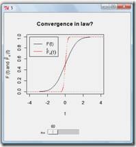
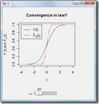
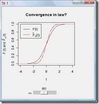
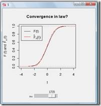
If you take a symmetrical random walk and scale the increments so that they are dependent on the time step, basically you get a Brownian motion. This can be easily checked by normalizing the series and validating against standard normal. The above graphs show that as you increase the time steps for a given T, scaled random walk divided by the variation, converges in distribution to standard normal.

Basic properties of BM are introduced where there is a special mention of quadratic variation converges to T.

The whole ram kahani of Brownian Motion and Brownian Bridge leads to the concept of Functional of Brownian Motion which is used heavily in Unit root testing. So, if you are a math fin student trying to read stochastic calculus, my humbe suggestion is not to miss “Brownian Bridge” at any cost as it is used in a lot of applications.

Chapter 7 : Brownian Motion Differentiation and Integration

If you compress Stochastic Calculus by Shreve in to 30 odd pages removing most of the math and present it in a completely intuitive sense, then you basically have this chapter in print. The chapter highlight the limitations of Reimann Calculus and shows that Brownian Motion calculus is a different animal where everything is a Lebesgue integral. So, in that sense this is quick recap of Ito’s calculus, Brownian Bridge , etc which are all very important to understand any unit root test , starting from the basic Dickey Fuller.

FINALLY , the chapter on Unit Roots 

Chapter 8 : Some examples of Unit Root Tests

This is the core of the book even though this is last chapter of the book. As mentioned earlier, the first 7 chapters is to prepare a reader to understand the material in this chapter.

There are basically two statistics that are typically used. Normalized bias and Pseudo t statistic. Normalized bias is powerful than pseudo t statistic but the latter is much better than the former whenever the error process has a correlated structure

The usage of Functional Central Limit Theorem is something any first timer would notice. The connection between Brownian Bridge and pseudo t statistic will be a revelation for people who just use some black box to test stationarity of the series / who do a quantile plot to show stationarity or the lack of it. Basically depending on whether you are testing a series which reverts to 0 or reverts to a constant or has a linear trend, the limiting distribution converges in distribution to various forms of Brownian Bridge. Most of them do not have closed forms and hence simulation procedures are resorted to understand the stationarity aspect.

All the p values for the t statistics are available in the paper by Dickey ( 1979). However the basic form of Dickey ( 1979) does not address lags. Hence augmented Dickey Fuller test is used. MacKinnon tables are also used .. But one thing to keep in mind is that , all these tests are basically  unit root tests where the null is non stationary and alternate is stationary. So, if you are basically trying to trade a spread, it is better to establish stationarity using KPSS type of test where the null is stationary and alternate is non stationary. Thus you are using two tests , firstly the unit root test which has null : Non stationary , alternate: stationary.. secondly , KPSS where null = stationary ; alternate = non stationary. So, your test should show that you reject null in unit root test and accept null in KPSS test ..Only then you have something that is tradable.

Elliott–Rothenberg–Stock Test for Unit Roots is also mentioned in a very detailed manner which basically improve the power of unit root tests.

Personally the non parametric test mentioned at the fag end of the book has been a great learning.  The idea is straightforward but the math needs to be understood carefully. The basic idea is this :

If you have a random walk with out drift and you estimate the test statistic relating to level crossing times for a specific (s), it converges in distribution to a folded standard normal distribution. If the random walk has a drift, the test statistic relating to the level crossing times converges in distribution to Rayleigh Distribution.  If the error has a correlation structure , one needs to detrend and the test statistic again converges in distribution to Rayleigh. I will definitely this soon as I am particularly inclined to use semi-parametric type of statistics than using only parametric stats.

  Takeaway:

This book is a great bridge between “having an intuitive notion of unit root” and  “having an in depth knowledge of various unit root tests that you can create your own unit root test ”.