This blog post summarizes the book titled “Getting Started with Google Bert”, by Sudharshan Ravichandran

Context

NLP research output from Google has created an revolution in NLP. Since the time word2vec came out in 2013, there have been innovative developments in this field at regular intervals. The models are getting bigger and better. This has of course created massive enthusiasm in the field and has further spawned research from companies like OpenAI, Facebook. This has also changed the research focus at many educational institutions where the researchers are actively putting their models to test and competing on publicly available leader-boards that give performance metrics of various models against standard datasets.

For a traditional quant, who does not have a background in NLP, it is a steep learning curve to understand various concepts relating to this subject. However with the recent developments in NLP, there has been an surge of literature for educating the “rest of us” on the theoretical and practical aspects of NLP. This book by Sudarsan Ravichandran, is one of those resources that can help a newbie, get up to speed on using pretrained models.

It was almost two years ago that I started my NLP journey. Needless to say, the intention was not to become an NLP expert but to understand just enough so that it could complement my existing skills and apply it to a few practical problems. BERT Model was one area that I found that difficult to understand. The paper on BERT was something I struggled to understand as it had a lot of implicit pre-requisites that were expected from a reader . There are many resources that have helped me in getting a good understanding of BERT. This is one of the newer books on BERT that is well written and can help the reader ease in to the various concepts and flatten the learning curve. Given that I had slogged through understanding ideas in NLP in the Pre-BERT era, this book was fairly easy to read through. The first 200 pages served as a recap of all the ideas that I had come across in blogs, articles, videos. In that sense, the book serves as a amalgamation of all the concepts needed to get a practical understanding of BERT. In this post, I will try to summarize the main points of the book

A Primer on Transformers

If you want to understand the math behind any model, your first stop might be the paper that goes in to the details OR some blog post that does a great job of distilling the main aspects of the model. The paper titled “Attention is all you need”, is probably one of the most widely cited papers in the last few years, in the context of NLP architecture. However the paper is not an easy read, at least for some one who is not incredibly familiar with the NLP concepts. The paper assumes some knowledge of RNN, encoder-decoder architecture, basic neural network architectures etc. It is likely that reading through this paper might seem pretty challenging and you might look for resources that explain the ideas of the attention mechanism. Jay Allamar, is one such person, who has managed to explain the workings of NLP models with fantastic visuals. His illustrations have been widely cited by many people, while introducing the work on transformers. His visual write-ups are one of the best ways to understand the attention framework. Chris McCormick series on BERT is also a wonderful way to get a familiarity of transformer architecture and BERT. The reason I am mentioning the above resources is that I still believe they are best places to start, for a newbie. One should go over this chapter AFTER one is reasonably comfortable with the basic idea of transformer architecture. I could be biased because that was the route I have followed. However I have a strong feeling that if someone who doesn’t have any clue on Transformers, might find the intro a little bit daunting, especially with so many NLP related concepts introduced all in one chapter.

I found the first chapter extremely useful in the sense that, it reinforced my earlier understanding of the transformer architecture. Like I said, the first encounter with a transformer architecture, for a newbie, is most likely going to be daunting, when he/she sees the following architecture

How does one go about understanding the various components of the above diagram? The first chapter does a fantastic job of pulling apart the architecture and explaining everything in detail with a few simple examples. The way the author explains these components is, by posing a set of questions along the way, so that the reader pauses at frequent intervals, primes his/her mind in order to understand the description of the components. By the end of the chapter, any attentive reader will have all the following questions answered:

• Why do we need self-attention in the first place, while building a language model ?
• How is self-attention implemented via query, key and value matrices ?
• What is scaled dot product attention ?
• What is the relevance of multi-headed attention ?
• What is the input to a transformer architecture?
• What is positional encoding of input sentence?
• What is the use of add and norm component in an encoder/decoder block?
• What is masked self-attention ? Why does one need to use it in a decoder block ?
• What is encoder-decoder attention and how should the math be different in terms of implementing it ?
• What are the inputs to encoder-decoder attention layer ?
• How are the query, key and value matrices different in encoder-decoder attention block as compared to self-attention block ?

A few other questions that are equally important that are listed below are also important, that might require you to hunt around other resources:

• What problem does self-attention solve, as compared to previous architectures ?
• Which was the first model that made heavy use of attention mechanism?
• What are the advantages of transformer architecture as compared to RNN’s and LSTM’s ?
• Is self-attention technique used in any other domain ? Finance/Econometrics
• What makes the transformer architecture suited for parallel processing?
• What is the performance of “transformer-architecture” based models in machine translation tasks? Do they have a higher BLEU score as compared to older models?
• What are the limitations of transformer architecture ?

Understanding the BERT Model

A pre-requisite to understanding BERT is the transformer architecture, a topic that is covered in the very first chapter in the book. The second chapter is more about understanding the tweaks that were done to make BERT a powerful NLP model. This chapter walks a reader through BERT in great detail, again through the use of simple examples. The main idea is that one takes the encoding layer of the “transformer” architecture, trains it on certain tasks such as masked language modeling and next sentence prediction, obtains a language model that can be used for a ton of downstream tasks. On the github site, as of today, there are many variants of BERT models mentioned:

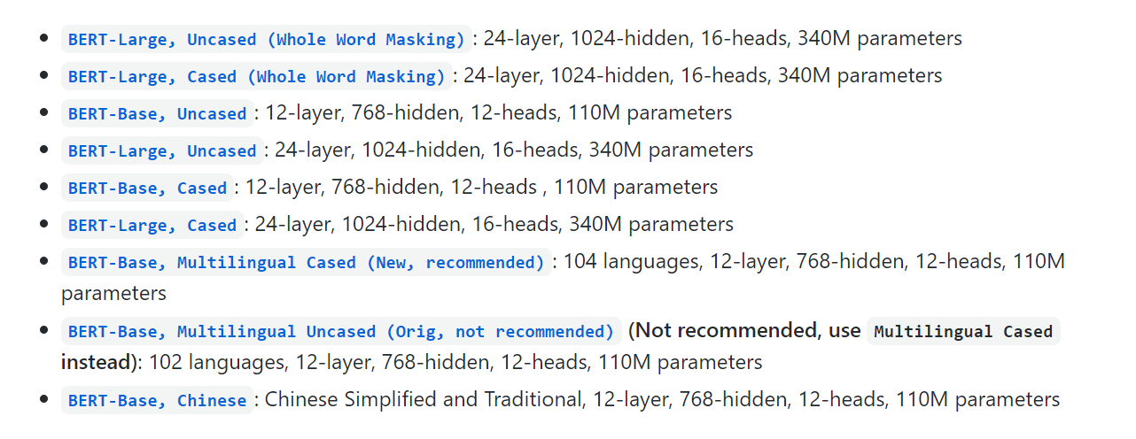
As one can see, one of the first things that differentiate among models are

• Number of encoder layers
• Number of attention heads
• Hidden Unit

For example BERT-base comprises 12 encoder layers, each stacked one on top of the others. All the encoders use 12 heads and the feedforward network in the encoder consists of 768 hidden units

The first thing that one must know about BERT is - what does it expect as an input ? Well, it expects three inputs for any sentence of pair of sentences

• Token embeddings
• Segment embeddings
• Position embeddings

How does one obtain the above embeddings ? The segment and position embeddings are straightforward, but token embeddings are tightly coupled with the vocabulary used to train the model. In the case of BERT, a special tokenizer called WordPiece tokenizer has been used. It is better to have a good understanding of the WordPiece and I highly recommend the BERT embeddings tutorial by Chris McCormick. Once you get your hands dirty with analyzing the various aspects mentioned in the tutorial, the contents of this chapter become very easy to understand and digest.

One of the most important differences between the usual word2vec embeddings and BERT embeddings is the use of subword embeddings. The chapter talks about three types of embedding algos

• Byte pair encoding(BPE): Take a frequency distribution of all words in the corpus, decide a vocab size, split the words in to multiple subwords having varying lengths. A single word might give rise to multiple subwords. Systematically select the subwords based on their frequency count in their corpus
• Byte Level Byte pair encoding(BBPE): Same as BPE but uses byte sequence of the converted word
• WordPiece: Works similar to BPE but the way we agglomerate the vocab is based on probabilities and not on frequency counts

Chapter Takeaways

The chapter does a good job of explaining all the internals of BERT. By the end of the chapter, a reader would be fairly comfortable in answering all the following questions:

• What is the vocabulary size of BERT ?
• How does BERT handle out-of-vocab words ?
• What is sub word tokenization ?
• What are the types of sub word tokenization algorithms ?
• What is Bidirectional about BERT ?
• What is the difference between auto-regressive and auto-encoding language models ?
• In Masked Language Modeling task, what is 80%-10%-10% rule that has been used ?
• There are various variants of BERT models. Some of them used Whole Word masking. What does it mean ?
• What is BERT trained on ?
• What does one mean by warm-up step ?
• What activation function does BERT use ?
• How id GELU different from ReLU?
• What is Byte pair encoding ?
• What is Byte-level byte pair encoding?
• What sub-word tokenization is used in BERT ?

Getting Hands-On with BERT

It is pretty easy to get started with transformers library from HuggingFace. Let’s say that you have a sentence, Getting Started with Google BERT. The library provides BertTokenizer and BertModel that can be readily used to obtain the input and output of a typical BERT model

• By using tokenizer function, you can obtain the token embeddings, attention masks and token type ids that can be sent as input to the BERT model
• The output of the model, i.e last hidden state, pooler output, hidden state output of all encoders, attention matrices, can be obtained by a few lines of code
• pooler_output can be used in further downstream processing as the representation of the entire sentence

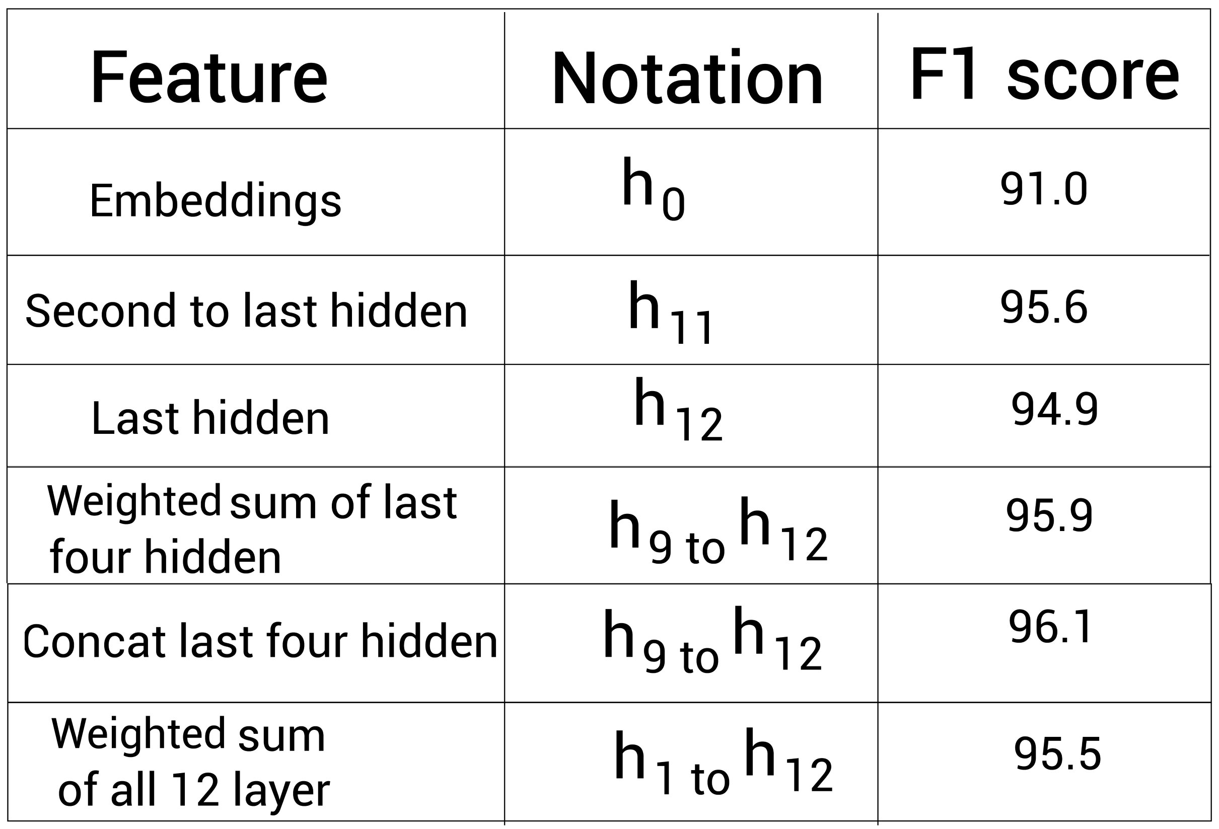
A question that one might have is, what is the use of hidden layer outputs ? Can they be used ? One can look at the performance metrics based on Google’s published results and take a cue that that hidden layers contain useful information and can be used in further downstream tasks.

Using Hugging Face

The following shows a code snippet that abstracts away all the complexity behind BERT:

 1
 2
 3
 4
 5
 6
 7
 8
 9
10
11
12
13
14
15
16
17

sentence = "Getting Started with Google BERT"
tokenizer = BertTokenizer.from_pretrained("bert-base-uncased")
encoded_sentence = tokenizer(sentence, return_tensors="pt")
input_ids = encoded_sentence["input_ids"]
attention_mask = encoded_sentence["attention_mask"]
token_type_ids = encoded_sentence["token_type_ids"]
model = BertModel.from_pretrained(
    "bert-base-uncased", output_attentions=True, output_hidden_states=True
)
output = model(
    input_ids=input_ids, attention_mask=attention_mask, token_type_ids=token_type_ids
)
metrics = {'last_hidden_state_shape':output.last_hidden_state.shape,
 'output.pooler_output.shape':output.pooler_output.shape,
 'len(output.hidden_states)':len(output.hidden_states),
 'len(output.attentions)':len(output.attentions)}
pd.Series(metrics)

1
2
3
4
5

last_hidden_state_shape       (1, 7, 768)
output.pooler_output.shape       (1, 768)
len(output.hidden_states)              13
len(output.attentions)                 12
dtype: object

As one can see, using a given model is pretty easy, thanks to transformers library. Which pretrained model should one use? There is no straightforward answer to this question as one might have to tirelessly experiment with many models and choose the one that fits the usecase. Huggingface has thousands of models for various training tasks. BERT alone has many variants

What can the BERT model be used for ? There are a couple of ways to use BERT based on the use case, that you have in mind.

• Use BERT as a feature extractor: Obtain the encoding layer stack’s output as a feature in a machine learning model
• FineTune for Classification: Use the [CLS] vector representation and feed in to a feedforward layer for classification task. Run the training for a few epochs so that all the weights of the model have a chance to get updated
• Question Answering: Use the [CLS] vector and perform a dot product with the starting position vector and ending position vector, do a softmax operation and obtain the span in the paragraph that best answers the question
• NER: Use the entire sentence representation at the final hidden layer, pass it through a classifier label that performs named entity recognition

The chapter uses fairly new version of transformers library and hence is very useful. However it misses out on auto classes, AutoModel, AutoTokenizer, AutoConfig, that make it easy to plug and play various NLP models, including the many BERT variants, that can be configured by specifying checkpoint strings.

Finetuning BERT for poems data

Here is a sample code that can be used to train a classifier

 1
 2
 3
 4
 5
 6
 7
 8
 9
10
11
12
13
14
15
16
17
18
19
20
21
22
23
24
25
26
27
28
29
30
31
32
33
34
35
36
37
38
39
40
41
42
43
44
45
46
47
48
49
50
51
52
53
54
55
56
57
58
59
60
61
62
63
64
65
66

# Load the tokenizer
from datasets import load_dataset, load_metric
import numpy as np
import numpy as np
from sklearn.metrics import accuracy_score, recall_score, precision_score, f1_score
from transformers import AutoTokenizer
from transformers import (
    AutoTokenizer,
    AutoConfig,
    AutoModelForSequenceClassification,
    DataCollatorWithPadding,
)
from transformers import TrainingArguments, Trainer
tokenizer = AutoTokenizer.from_pretrained("bert-base-uncased")
# Load the dataset
poems = load_dataset("poem_sentiment")
poems = poems.filter(lambda x: x["label"] in [0, 1, 2])
poems = poems.map(
lambda x: tokenizer(x["verse_text"], truncation=True, max_length=512), batched=True
)
poems = poems.remove_columns(["id", "verse_text"])
# Load the model
cfg = AutoConfig.from_pretrained("bert-base-uncased")
cfg.num_labels = 3
model = AutoModelForSequenceClassification.from_config(cfg)
data_collator = DataCollatorWithPadding(tokenizer)
batch_size = 32
epochs = 1
# Load the metric
metric = load_metric("accuracy")
def compute_metrics(eval_pred):
logits, labels = eval_pred
predictions = np.argmax(logits, axis=-1)
return metric.compute(predictions=predictions, references=labels)
# Prepare training arguments
training_args = TrainingArguments(
output_dir="./results",
evaluation_strategy="epoch",
num_train_epochs=epochs,
per_device_train_batch_size=batch_size,
per_device_eval_batch_size=batch_size,
learning_rate=1e-4,
logging_dir="./logs",
)
# Instantiate the trainer
trainer = Trainer(
model,
training_args,
train_dataset=poems["train"],
eval_dataset=poems["test"],
compute_metrics=compute_metrics,
tokenizer=tokenizer,
data_collator=data_collator,
)
# Train the model
trainer.train()

Chapter Takeaways

This chapter comes in right after covering adequate theoretical aspects of the model. I like the fact that this chapter is not relegated to some appendix or somewhere towards the end of the book. By making the reader go through the relevant code, the author makes sure that the concepts have sinked in for the reader and the reader is ready to plunge in to other variants of NLP models.

Bert Variants I - ALBERT, RoBERTa, ELECTRA and SpanBERT

ALBERT

Stands for A Lite version of BERT. The name suggests that this model is more lightweight but in what sense? The chapter introduces two main features of ALBERT that makes it different from BERT

• Cross-layer parameter sharing: This involves sharing the parameters of the first encoding layer with all the other layers in the encoding stack. There are variants, based on the shared layers
  • All-shared - Share all layers of the first encoder with all other encoders
  • Shared feedforward network: Share only the feedforward parameters of the first encoder with the other encoders
  • Shared Attention: Share only the attention layer of the first encoder with all the rest of encoder layers in the stack
• Factorized embedding layer parameterization: This feature is mainly introduced to make the hidden layer dimension decoupled form the input encoding dimension

As one can see, a different learning task has been used - SOP(Sentence Order Prediction). It has been observed that NSP(Next Sentence Prediction) task is not really useful and hence researchers behind ALBERT have used SOP task. This is a task that involves the model deciding whether sentence order is correct/swapped.

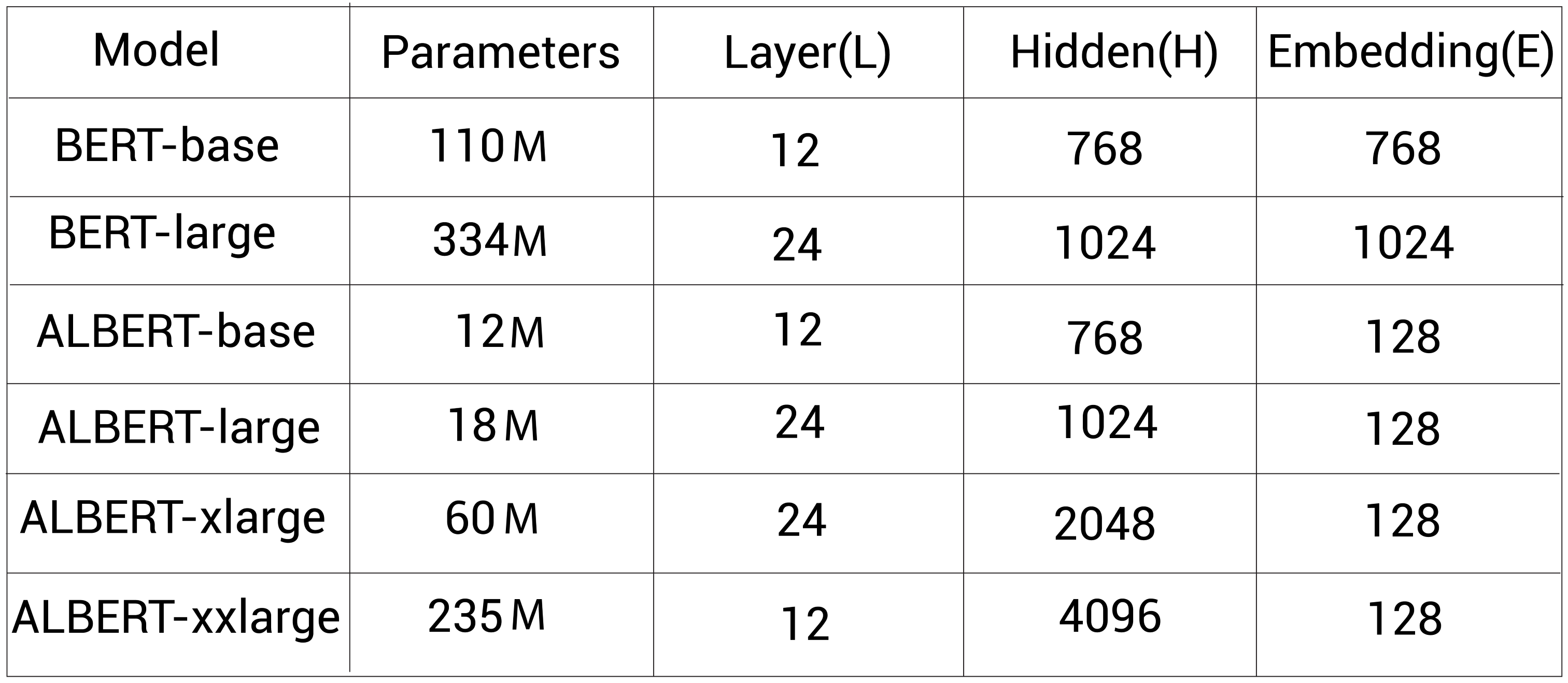
The following gives the comparison of BERT with ALBERT variants

Sample code using Hugging Face

1
2
3
4
5
6
7

model = AutoModel.from_pretrained('albert-base-v2')
tokenizer = AutoTokenizer.from_pretrained('albert-base-v2')
inputs = tokenizer("Getting started with Google BERT", return_tensors="pt")
output = model(**inputs)
metrics = {'last_hidden_state_shape':output.last_hidden_state.shape,
 'output.pooler_output.shape':output.pooler_output.shape}
pd.Series(metrics)

1
2
3

last_hidden_state_shape       (1, 7, 768)
output.pooler_output.shape       (1, 768)
dtype: object

RoBERTa

Stands for Robustly Optimized BERT pre-trained Approach. The following are some of the aspects that are different from BERT

Dynamic masking means instead of using a single masked sentence that goes through all the training epochs, we mask the same sentence in different ways and train the network using different variations of maskings, for the same input sentence. So, what exactly is the input to RoBERTa ? The idea here is to train BERT without NSP task and the input consists of a full sentences, which is sampled continuously from one or more documents. The input consists of at most 512 tokens. If we reach the end of one document, then we begin sampling from the next document.

Sample code using Hugging Face

1
2
3
4
5
6
7

model = AutoModel.from_pretrained('roberta-base')
tokenizer = AutoTokenizer.from_pretrained('roberta-base')
inputs = tokenizer("Getting started with Google BERT", return_tensors="pt")
output = model(**inputs)
metrics = {'last_hidden_state_shape':output.last_hidden_state.shape,
 'output.pooler_output.shape':output.pooler_output.shape}
pd.Series(metrics)

1
2
3

last_hidden_state_shape       (1, 8, 768)
output.pooler_output.shape       (1, 768)
dtype: object

ELECTRA

Stands for Efficiently Learning An Encoder that Classifies Token Replacements. The following are some of the aspects that are different from BERT

Sample code using Hugging Face

1
2
3
4
5
6

model = AutoModel.from_pretrained("google/electra-small-discriminator")
tokenizer = AutoTokenizer.from_pretrained("google/electra-small-discriminator")
inputs = tokenizer("Getting started with Google BERT", return_tensors="pt")
output = model(**inputs)
metrics = {"last_hidden_state_shape": output.last_hidden_state.shape}
pd.Series(metrics)

1
2

last_hidden_state_shape    (1, 7, 256)
dtype: object

SpanBERT

Used for tasks such as question answering wehre we need to predict the span of the text The following are some of the aspects that are different from BERT

Sample code using Hugging Face

 1
 2
 3
 4
 5
 6
 7
 8
 9
10

model = AutoModel.from_pretrained("SpanBERT/spanbert-base-cased")
tokenizer = AutoTokenizer.from_pretrained("SpanBERT/spanbert-base-cased")
inputs = tokenizer("Getting started with Google BERT", return_tensors="pt")
output = model(**inputs)
output.keys()
metrics = {
    "last_hidden_state_shape": output.last_hidden_state.shape,
    "output.pooler_output.shape": output.pooler_output.shape,
}
pd.Series(metrics)

1
2
3

last_hidden_state_shape       (1, 10, 768)
output.pooler_output.shape        (1, 768)
dtype: object

1
2
3
4
5
6
7
8
9

qa_pipeline = pipeline(
    "question-answering",
    model="mrm8488/spanbert-finetuned-squadv2",
    tokenizer="SpanBERT/spanbert-base-cased",
)
results = qa_pipeline({ 'question': "What is machine learning?",
                        'context': """Machine learning is a subset
                        of artificial intelligence. It is widely for creating a variety of applications such as email filtering and computer vision""" })
"" .join(results['answer'])

1

a subset of artificial intelligence

Bert Variants II - Based on Knowledge Distillation

Power of BERT comes from its millions of parameters in its unique architecture. The same power becomes a limitation for other use cases where one can’t tolerate high inference times. That’s where knowledge distillation comes in. We can transfer the knowledge form a large pre-trained BERT to a small BERT.

Knowledge Distillation

It is a model compression technique in which a small model is trained to reproduce the behavior of a large pre-trained model. It is also referred to as teacher-student learning, where the large pre-trained model is the teacher and the small model is the student. The idea of softmax temperature is illustrated well via a simple example mentioned in the chapter

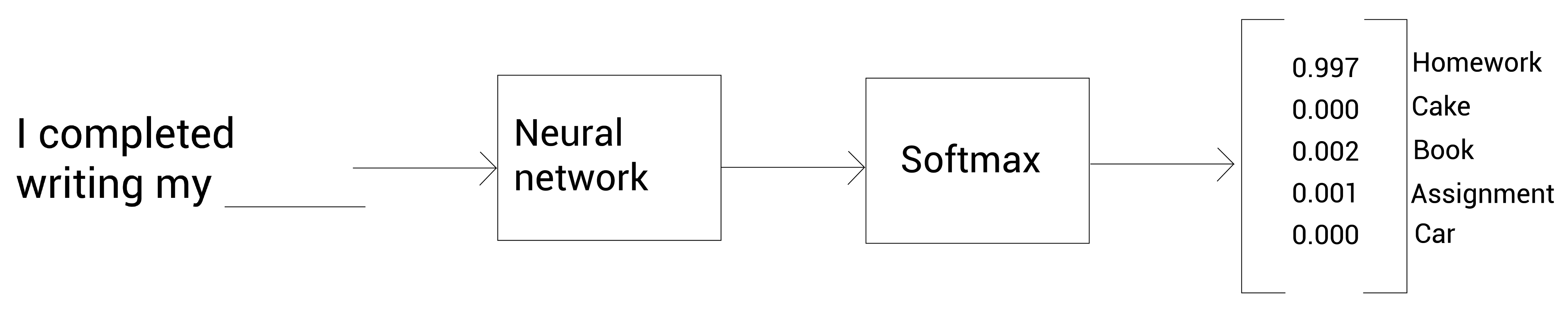
The key idea is

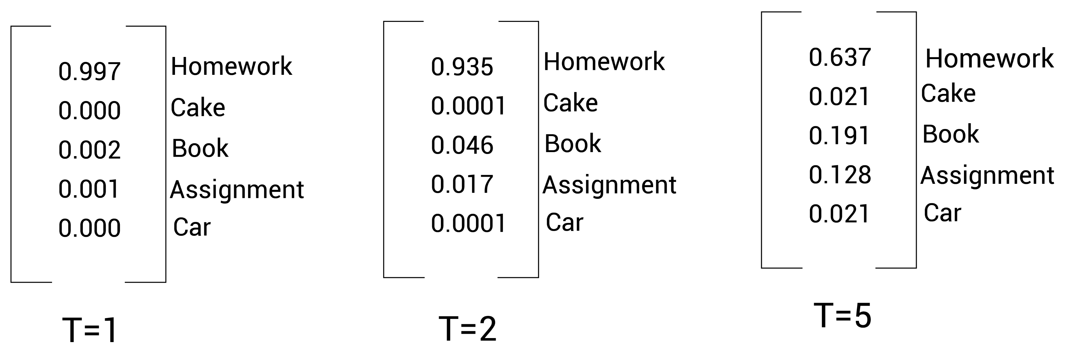
With softmax temperature, we can obtain the dark knowledge. First, we pretrain the teacher network with softmax temperature to obtain dark knowledge. Then, during knowledge distillation(transferring knowledge from the teacher to the student), we transfer this dark knowledge from the teacher to the student

The sample architecture of a teacher-student is illustrated below

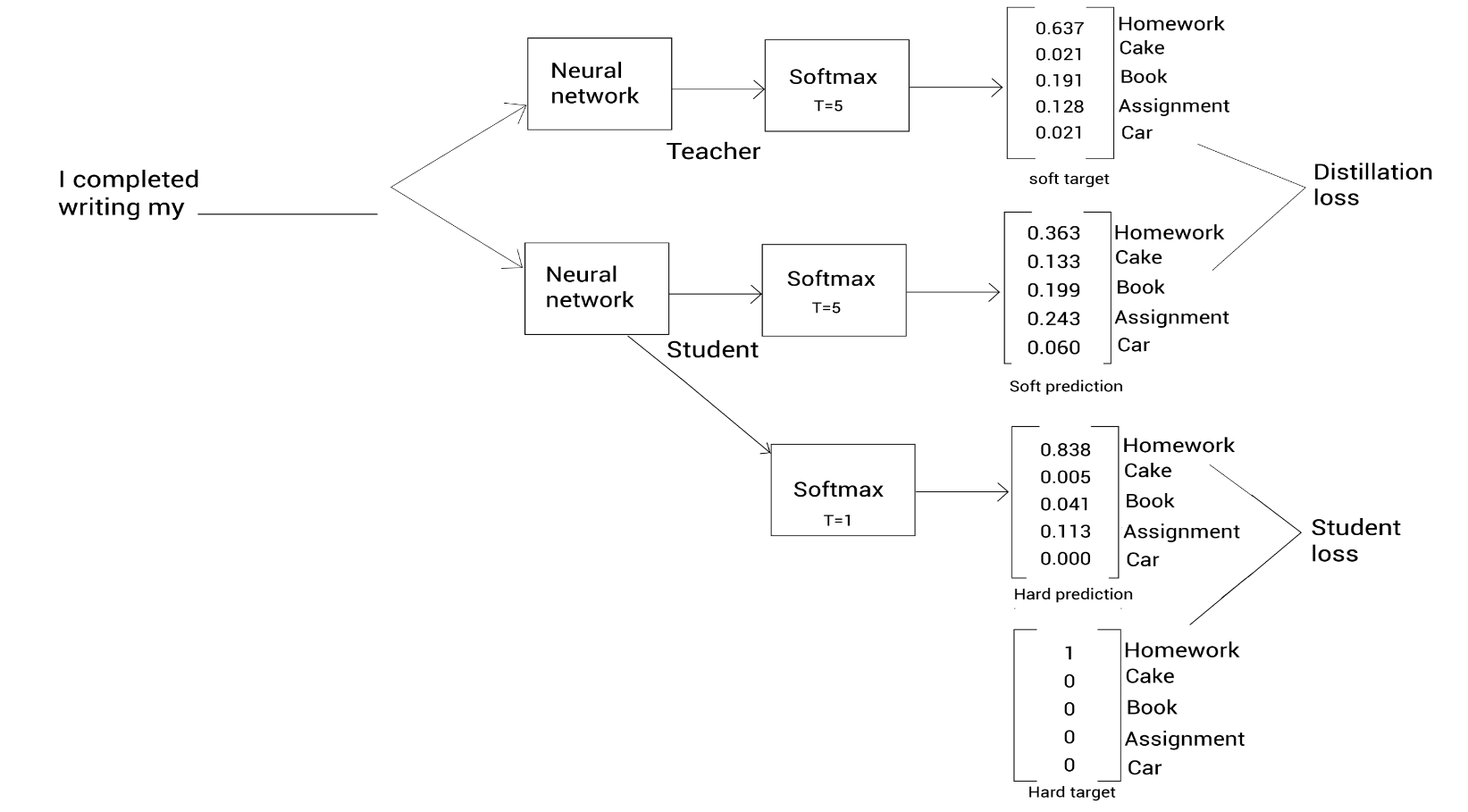
In the above architecture, the idea is to align soft target with soft prediction. The cross-entropy loss between the soft target and soft predication is also called the distillation loss. One should take in to consideration student loss, which is the cross-entropy loss between the hard target and hard prediction.

In Knowledge distillation, we take the pre-trained network as the teacher network. We train the student network to obtain knowledge from the teacher network through distillation. We train the student network by minimizing the loss, which is the weighted sum of student and distillation loss.

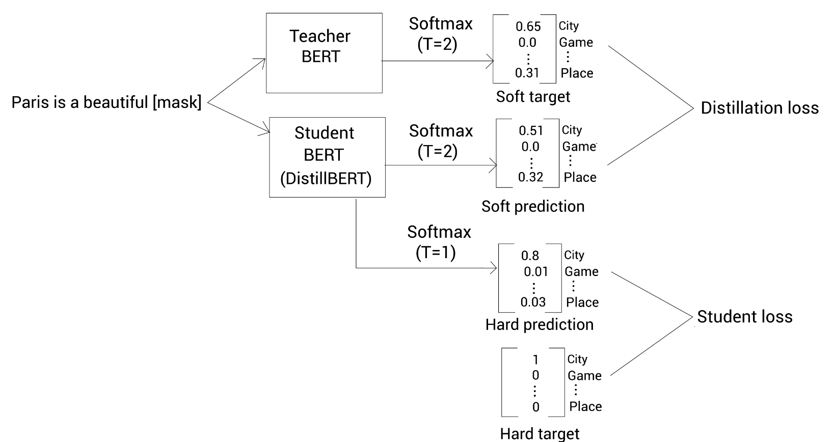
DistilBert

The pre-trained BERT model has a large number of parameters and also high inference time, which makes it harder to use on edge devices such as mobile phones. To solve this issue, Hugging Face created DistilBert that is a smaller, faster, cheaper and lighter version of BERT. The large pre-trained BERT is called a Teacher BERT and the small BERT is called a Student BERT

DistilBert is 60% faster and 40% smaller compared to large BERT models. It gives almost 97% accurate results as the original BERT-base model. DistilBERT was trained on eight 16 GB V100 GPUs for 90 hours.

The basic ideas of student-teacher architecture is used to showcase the main components of DistilBert

The following are some of the aspects of the model:

Sample code using Hugging Face

The code for classification using DistilBERT follows almost the same template as that of any model

 1
 2
 3
 4
 5
 6
 7
 8
 9
10
11
12
13
14
15
16
17
18
19
20
21
22
23
24
25
26
27
28
29
30
31
32
33
34
35
36
37
38
39
40
41
42
43
44
45
46
47
48
49
50
51
52
53
54
55
56
57
58
59
60
61
62
63
64

from datasets import load_dataset, load_metric
import numpy as np
import numpy as np
from sklearn.metrics import accuracy_score, recall_score, precision_score, f1_score
from transformers import AutoTokenizer
from transformers import (
    AutoTokenizer,
    AutoConfig,
    AutoModelForSequenceClassification,
    DataCollatorWithPadding,
)
from transformers import TrainingArguments, Trainer
# Load the tokenizer
tokenizer = AutoTokenizer.from_pretrained("distilbert-base-uncased")
# Load the dataset
poems = load_dataset("poem_sentiment")
poems = poems.filter(lambda x: x["label"] in [0, 1, 2])
poems = poems.map(
lambda x: tokenizer(x["verse_text"], truncation=True, max_length=512), batched=True
)
poems = poems.remove_columns(["id", "verse_text"])
# Load the model
cfg = AutoConfig.from_pretrained("distilbert-base-uncased")
cfg.num_labels = 3
model = AutoModelForSequenceClassification.from_config(cfg)
data_collator = DataCollatorWithPadding(tokenizer)
batch_size = 32
epochs = 3
# Load the metric
metric = load_metric("accuracy")
def compute_metrics(eval_pred):
logits, labels = eval_pred
predictions = np.argmax(logits, axis=-1)
return metric.compute(predictions=predictions, references=labels)
# Prepare training arguments
training_args = TrainingArguments(
output_dir="./results",
evaluation_strategy="epoch",
num_train_epochs=epochs,
per_device_train_batch_size=batch_size,
per_device_eval_batch_size=batch_size,
learning_rate=1e-4,
logging_dir="./logs",
)
# Instantiate the trainer
trainer = Trainer(
model,
training_args,
train_dataset=poems["train"],
eval_dataset=poems["test"],
compute_metrics=compute_metrics,
tokenizer=tokenizer,
data_collator=data_collator,
)
trainer.train()

TinyBERT

The key motivating question behind TinyBERT is, “Can one do a knowledge transfer from the other layers of the teacher BERT ?”. TinyBERT does exactly that.

In TinyBERT, apart from transferring knowledge from the output layer of the teacher to the student, we also transfer knowledge from embedding and encoder layers.

Here is the basic archicture of TinyBERT

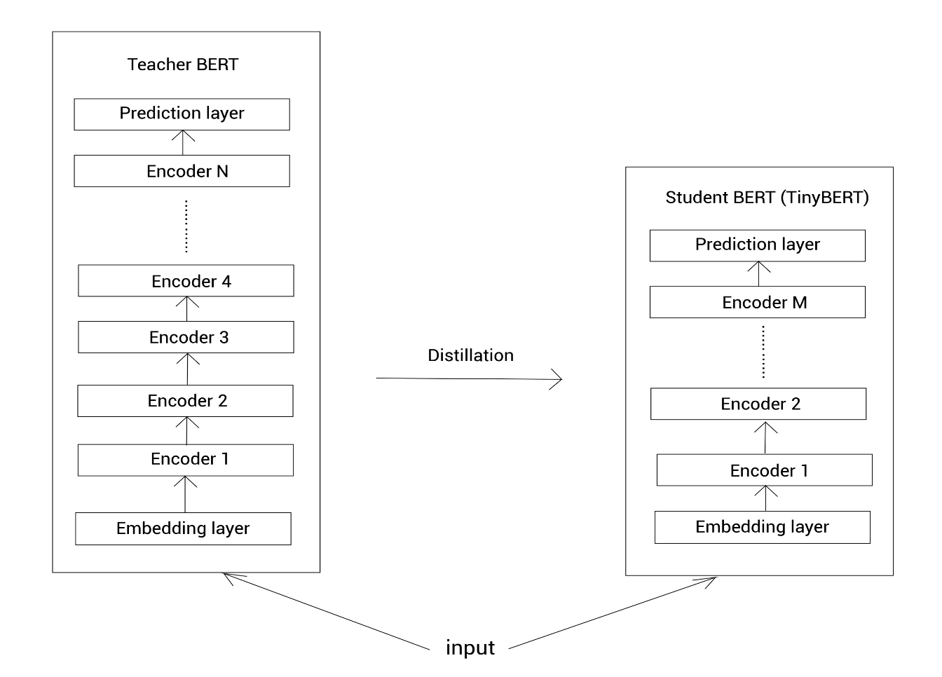
Transfer of knowledge happens at each of the three layers

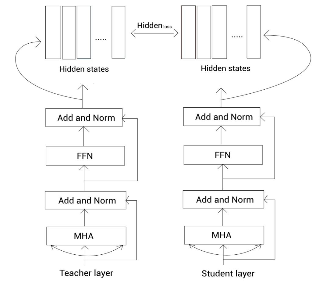
• Transformer layer
  • This comprise two types of distillation
    • Attention-based distillation

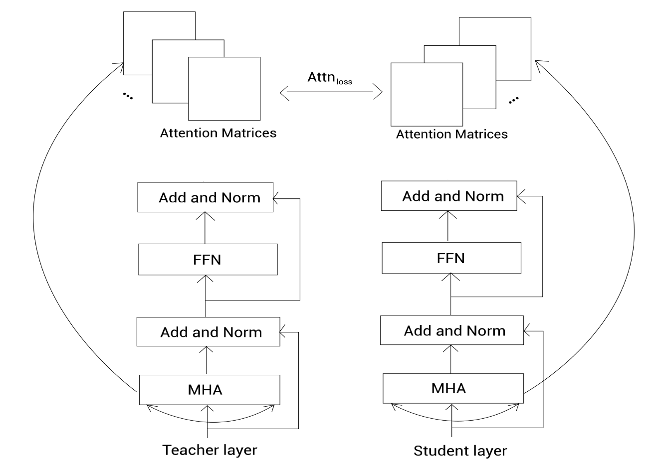
• Hidden state based distillation

• Embedding layer
• Prediction layer

Thus the loss function should encapsulate the loss in all the layers.

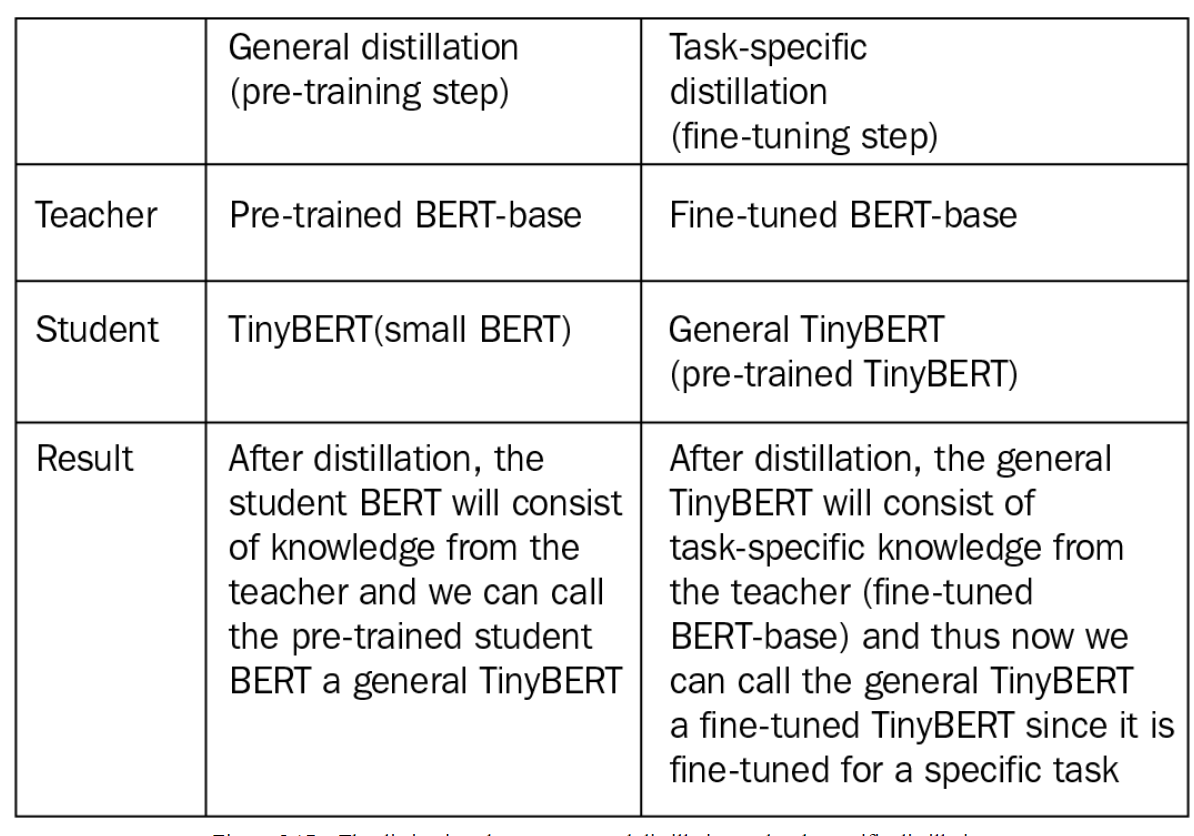
In training the student BERT, a two stage learning framework is followed:

• General distillation
• Task-specific distillation

The following aptly summarizes the difference

Transferring knowledge from BERT to Neural Networks

The basic idea behind this archicture is to take a finetuned BERT and transfer it to a general non-transformer based architecture such as Neural Networks. The framework that needs to be used for such a transfer is already covered in the previous sections. One computes the distillation loss, the student loss for the transfer and minimizes the loss function. There is one additional hack that is needed, i.e. way to increase the data for transferring the knowledge. This is done via data-augmentation process. There are three popoular methods for performing task-agnostic data augmentation:

• Masking
• POS-guided word replacement
• n-gram sampling

Chapter Takeaways

I found this chapter very interesting as I had never paid attention to mechanics of Distillation process. Given that I need to implement a usecase that needs quick inferencing, I will have to look in to distillation based models and compare the performance of bulky model vs distillation based models. There are already a few models that have been trained on the specific corpus of text that I am using for a project. Now there is an additional tasks that I need to do:

1. Does it make sense to use a bulky homegrown BERT family model ?
2. Would I be able transfer finetuned BERT to a LSTM for sentiment analysis ?
3. Will there be a trade-off in performance ?

All exciting questions that I hope to answer as I plod along.

Exploring BERTSUM for Text Summarization

Basic architecture

BERT model fine-tuned for the text summarization task is often called BERTSUM. I was reasonably familiar with this NLP task and found the contents of the chapter very interesting. My knowledge in this area was more around the classic old school way of approaching the problem of extractive summarization. If one has to use BERT for extractive or abstractive summarization, the first thing that one needs to think about is the input ? What should be the input to the BERT model? Unlike traditional sentence(s) input, summarization involves taking in to consideration multiple sentences. So, how does prepare segment embeddings for multiple sentences? The author does a good job of explaining the input preparation steps using a set of visuals

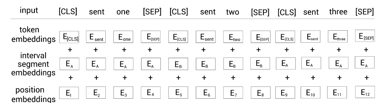
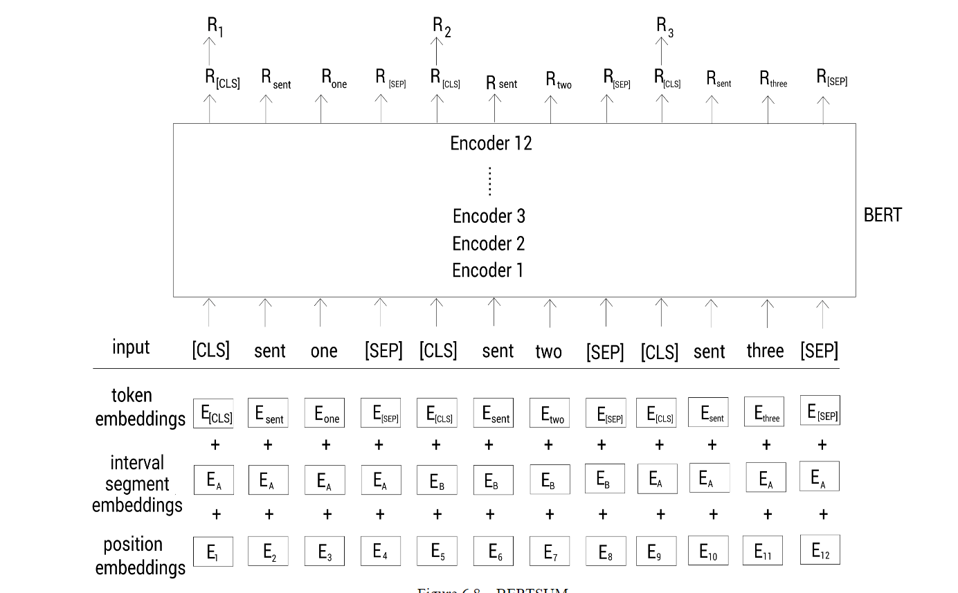
Why are we representing input tokens with additional [CLS] tokens at the beginning of every sentence? The main reason is that we want a sentence representative token for each of the sentence that we feed in.

BERTSUM with a classifier

The additional layer to be used is obvious, once we have the sentence representation of each sentence. Each of the sentence representations are sent in to a sigmoid layer that spits out the probability that the individual sentence is considered for summarization

BERTSUM with a transformer

One can add in more levels of sophistication by using the sentence representation with a transformer layer

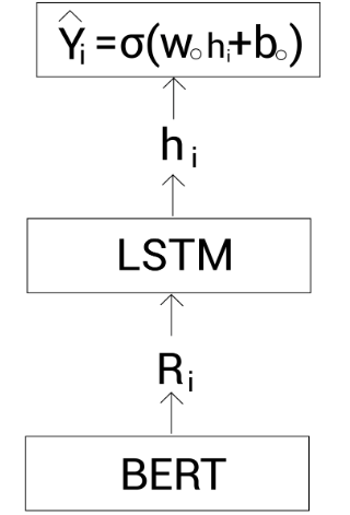
BERTSUM with LSTM

One can add in more levels of sophistication by using the sentence representation with a LSTM layer

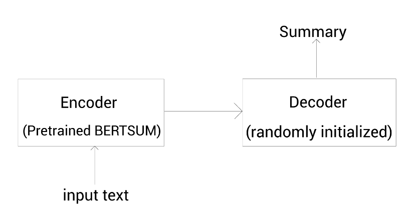
Abstractive summarization with BERT

In this type of summarization, one uses pre-trained BERT as the encoder layer and summarization as the decoder layer

ROUGE evaluations

This section of the chapter gives the details behind various evaluation metrics that can be used to evaluate summarization output. The following metrics are covered in detail:

• ROUGE-N
• ROUGE-L
• ROUGE-W
• ROUGE-S
• ROUGE-SU

Performance of BERTSUM model

The final section of the chapter gives the performance details of various BERTSUM model architectures

Applying BERT to other languages

Understanding Multilingual BERT

Multilingual BERT(M-BERT) is used to obtain the representations of text in different languages, other than just English. M-BERT is trained using Wikipedia text of 104 different languages. Since the representation of languages in Wikipedia is not uniform, certain sampling techniques are used that undersample high-resource languages and over sample low-resource languages.

The following table summarizes the main aspects of M-BERT:

Sample Hugging Face code

 1
 2
 3
 4
 5
 6
 7
 8
 9
10
11

model = AutoModel.from_pretrained("bert-base-multilingual-cased",output_attentions=True, output_hidden_states=True)
tokenizer = AutoTokenizer.from_pretrained("bert-base-multilingual-cased")
inputs = tokenizer("Getting started with Google BERT", return_tensors="pt")
model.eval()
with torch.no_grad():
    output = model(**inputs)
metrics = {'last_hidden_state_shape':output.last_hidden_state.shape,
 'output.pooler_output.shape':output.pooler_output.shape,
 'len(output.hidden_states)':len(output.hidden_states),
 'len(output.attentions)':len(output.attentions)}
pd.Series(metrics)

1
2
3
4
5

last_hidden_state_shape       (1, 8, 768)
output.pooler_output.shape       (1, 768)
len(output.hidden_states)              13
len(output.attentions)                 12
dtype: object

Evaluating M-BERT on NLI

In a typical Natural language inference task, the goal of any NLP model is to determine whether a hypothesis is an entailment, contradiction or underdetermined, given a premise. Thus, we feed a sentence pair to the model and it has to classify whether the sentence pair belongs to entailment, contradiction or is an undetermined class.

One can evaluate NLI under various settings

• Zero-shot
• Translate-Test
• Translate-Train
• Translate-Train-All

BERT performs well on all the above settings.

How multilingual is multingual BERT ?

The question that the author urges the reader to think about is,

How is M-BERT learning the representation across multiple languages without any specialized cross-lingual training and paired training set? How is M-BERT able to perform the zero-shot transfer? How multilingual is our M-BERT ?

Does the effectiveness of M-BERT come from the fact that there could be overlap of vocabulary across several languages? The author shows research output that dispels the notion of vocab overlap driving M-BERT effectiveness. Research findings show that M-BERT is powerful across languages that have similar typological features. For languages that do not have similar topological features like English-Japanese, M-BERT does not perform well. Also M-BERT can also handle code switched text but not transliterated text

Cross-Lingual Language Model(XLM)

BERT trained with a cross-lingual objective is referred to as cross-lingual language model(XLM).

The following table summarizes the main aspects of XLM:

It has been found that XLM trained using MLM and TLM performs better than XLM with only MLM. It has also been found that XLM performs better than M-BERT

XLM-R

XLM-R is basically an extension of XLM with a few modifications to improve performance. It stands for XLM-RoBERTa model and represents the state of the art for learning cross-lingual representation.

The following table summarizes the main aspects of XLM-R

Language specific BERT

The final section of this chapter walks the reader through monolingual BERT models that are available for various languages

• FlauBERT for French
• BETO for Spanish
• BERTje for Dutch
• German BERT
• Chinese BERT
• Japanese BERT
• FinBERT for Finnish
• UmBERTo for Italian
• BERTimbay for Portugese
• RuBERT for Russian

All the above models can be easily loaded and worked with the Auto classes available in the Hugging Face library

Exploring Sentence and Domain Specific BERT

Sentence BERT

This chapter takes the reader through exploring sentence similarity task, i.e. given a sentence, what is the most similar sentence to to it, from a corpus of sentences ? Shouldn’t it be a straightforward task: get the representation of the sentence from a pre-trained BERT and then check the distance between the input representation vis-a-vis sentence representations of all the sentences in the corpus? Well, the procedure makes sense, but it computationally slow. That’s where Sentence BERT comes in. Sentence BERT drastically reduces the inference time of BERT.

Firstly, how does one get sentence representation of Sentence BERT ? Taking the representation of [CLS] token is not going to be sufficient if we are not fine tuning BERT. The best way to get representation is via pooling(mean/max) the representation of all tokens.

Sentence-BERT uses Siamese network architecture, i.e. two parallel layers are fed a sentence, and the network can either be set up do a classification task or a regression task

• Classification Task : classify whether the sentences are similar/dissimilar

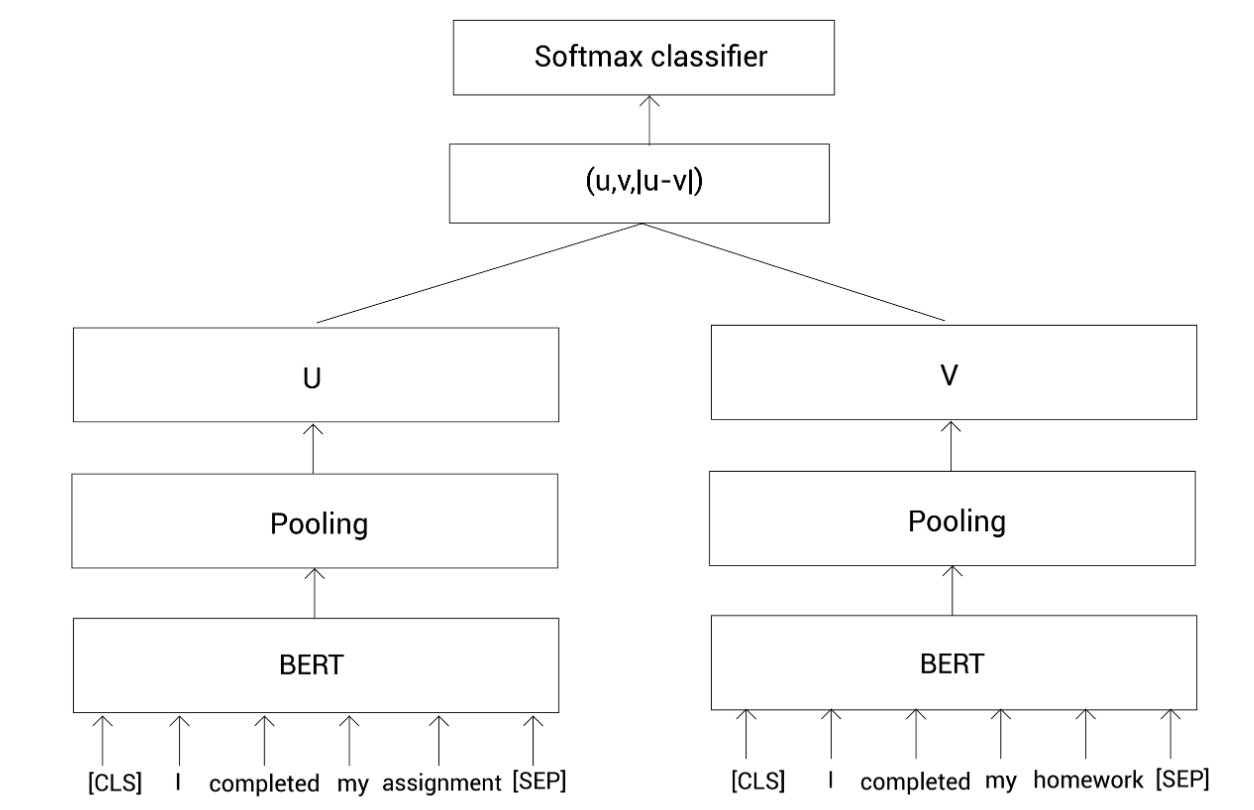
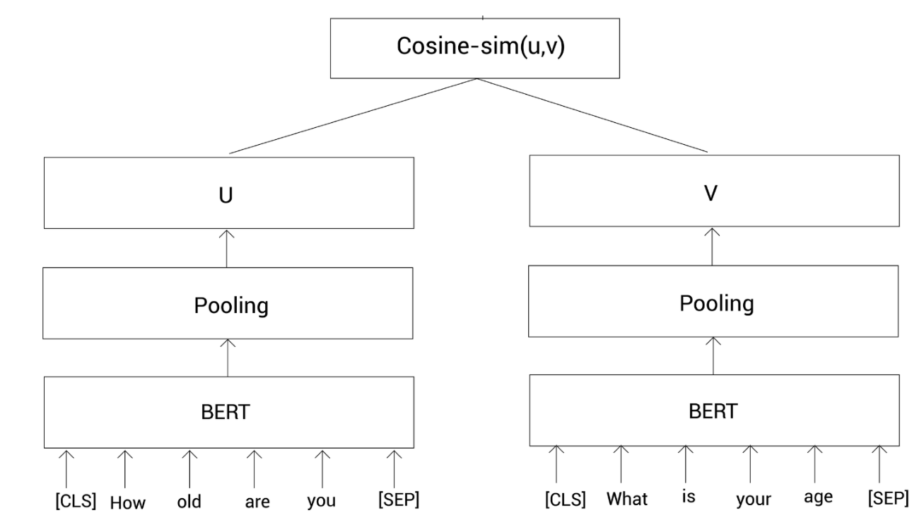
• Regression task: train the network to match the labeled similarity metric for pair of sentences

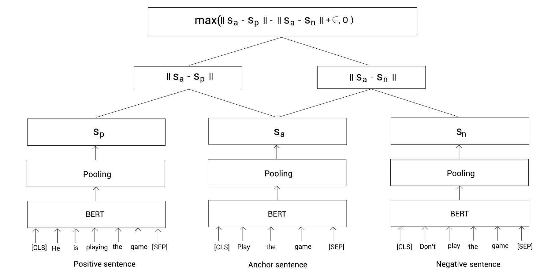
The above architecture can also be extended to triplenet architecture to perform the following task:

• Given an anchor sentence, positive sentence and negative sentence, fine tune a model so that similarity between anchor sentence and positive sentence is high and similarity between anchor sentence and negative sentence is low

The following architecture can be used to train a network:

Sample Hugging Face code

• Computing Sentence Representation

  1 2 3 4 5 6 7 8 9 10 11

  model = AutoModel.from_pretrained("sentence-transformers/bert-base-nli-mean-tokens") tokenizer = AutoTokenizer.from_pretrained("sentence-transformers/bert-base-nli-mean-tokens") inputs = tokenizer("I am enjoying this book", return_tensors="pt") model.eval() with torch.no_grad(): output = model(**inputs) metrics = { "last_hidden_state_shape": output.last_hidden_state.shape, "output.pooler_output.shape": output.pooler_output.shape, } pd.Series(metrics)

  1 2 3

  last_hidden_state_shape (1, 7, 768) output.pooler_output.shape (1, 768) dtype: object

• Computing Similarity

  1 2 3 4 5 6 7 8 9

  sentence_1 = tokenizer("I am enjoying this book", return_tensors="pt") sentence_2 = tokenizer("This book is well written", return_tensors="pt") model.eval() with torch.no_grad(): output_1 = model(**sentence_1) output_2 = model(**sentence_2) cos = torch.nn.CosineSimilarity(dim=1) cos(output_1['pooler_output'], output_2['pooler_output'])

  1	tensor([0.9568])

• Finding Similar sentence

  1 2 3 4 5 6 7 8 9 10 11 12 13 14 15 16 17 18 19

  inp_question = "When is my product getting delivered?" master_dict = [ "How to cancel my order?", "Please let me know about the cancellation policy?", "Do you provide refund?", "what is the estimated delivery date of the product?", "why my order is missing?", "how do i report the delivery of the incorrect items?", ] output_master = [] model.eval() with torch.no_grad(): output_1 = model(**tokenizer(inp_question, return_tensors="pt")) for sent in master_dict: output_master.append(model(**tokenizer(sent, return_tensors="pt"))) cos = torch.nn.CosineSimilarity(dim=1) output_master_pooled = [x['pooler_output'] for x in output_master] sim = cos(output_1["pooler_output"], torch.cat(output_master_pooled)) inp_question,master_dict[torch.argmax(sim).item()]

  1 2	When is my product getting delivered? Please let me know about the cancellation policy?

  The chapter also goes in to details about transferring the knowledge from a Monolingual sentence BERT to Multilingual sentence BERT

Domain specific BERT

The last section of the chapter goes in to the details behind Clinical BERT and BioBERT. Of course one can rely on vanilla BERT and use it for various domains but there will always be a case for training a BERT based on the domain specific pre-training data. There are two domain specific BERTs, clinical BERT and BioBERT that have been mentioned in the book. As far as training tasks are concerned, they are similar to BERT, the only difference is the training data. Needless to say, the fine tuned domain specific BERTs perform better than vanilla BERT on all measures, while evaluating on domain specific text.

Working on VideoBERT, BART and more

The last chapter is more a leisurely and an entertaining read about the possibilities of applying BERT to areas one might not immediately think of - use a set of videos as training data and learn the representation of language and video together. Once the model has been pre-trained, it can be used for downstream tasks such as image caption generation, video captioning, predicting the next frames of a video and similar applications. BART, the model for Facebook is also mentioned and the main features of the model are represented via visuals.

The final section of the chapter goes in to discussing two popular libraries for BERT, ktrain and bert-as-service

Takeaway

Kudos to the author, for putting in the effort to write the book. I have thoroughly enjoyed reading this book as it has just the right amount of technical details that are enough to grasp the complexities behind BERT. The book shines among all the books present on NLP because of the breadth of BERT variants that are thoroughly explained. Also, the fact that the book makes use of the newer version of transformers library makes it immensely useful to get to work right away.