Poisson Regression - Chap 4

> setwd("C:/Cauldron/garage/R/soulcraft/Volatility/Learn/Dobson-GLM")
> data <- read.csv("test7.csv", header = T, stringsAsFactors = F)
> plot(data$x, data$y, pch = 19, col = "blue", cex = 2)

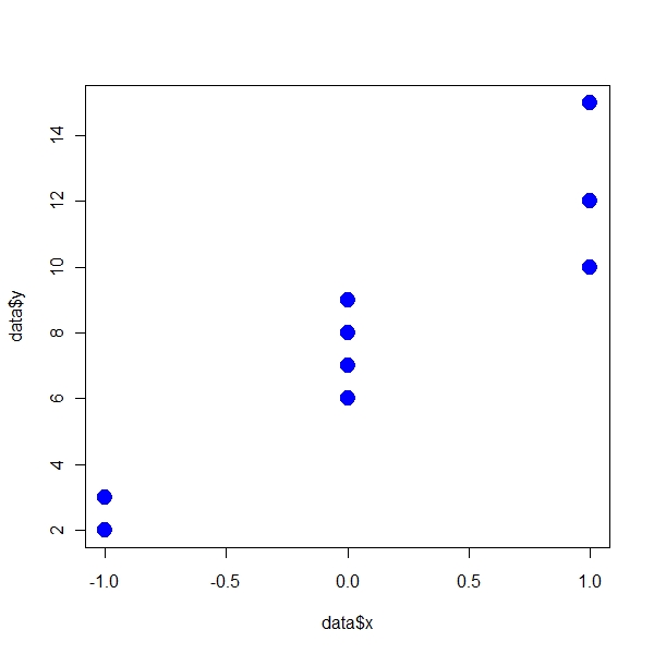
> beta0 <- c(7, 5)
> poisreg <- function(beta0) {
+     beta <- matrix(data = beta0, ncol = 1)
+     z <- matrix(data = data$y, ncol = 1)
+     W <- diag(9)
+     diag(W) <- 1/(X %*% beta)
+     X <- cbind(rep(1, 9), data$x)
+     LHS <- t(X) %*% W %*% X
+     RHS <- t(X) %*% W %*% z
+     beta.res <- solve(LHS, RHS)
+     return(beta.res)
+ }
> iterations <- matrix(data = NA, nrow = 2, ncol = 5)
> iterations[, 1] <- poisreg(beta0)
> for (i in 2:5) {
+     iterations[, (i)] <- poisreg(iterations[, (i - 1)])
+ }
> print(iterations)
         [,1]     [,2]     [,3]     [,4]     [,5]
[1,] 7.451389 7.451632 7.451633 7.451633 7.451633
[2,] 4.937500 4.935314 4.935300 4.935300 4.935300

> W <- diag(9)
> diag(W) <- 1/(X %*% iterations[, 4])
> X <- cbind(rep(1, 9), data$x)
> J <- t(X) %*% W %*% X
> Jinv <- solve(J)

> iterations[, 4]
[1] 7.451633 4.935300
> iterations[1, 4] + sqrt(Jinv[1, 1]) * 1.96 * c(-1, 1)
[1] 5.718750 9.184516
> iterations[2, 4] + sqrt(Jinv[2, 2]) * 1.96 * c(-1, 1)
[1] 2.800515 7.070085

> model.pois <- glm(data$y ~ data$x, family = poisson(link = identity))
> summary(model.pois)
Call:
glm(formula = data$y ~ data$x, family = poisson(link = identity))

Deviance Residuals:
    Min       1Q   Median       3Q      Max
-0.7019  -0.3377  -0.1105   0.2958   0.7184

Coefficients:
            Estimate Std. Error z value Pr(>|z|)
(Intercept)   7.4516     0.8841   8.428  < 2e-16 ***
data$x        4.9353     1.0892   4.531 5.86e-06 ***
---
Signif. codes:  0 '***' 0.001 '**' 0.01 '*' 0.05 '.' 0.1 ' ' 1

(Dispersion parameter for poisson family taken to be 1)

    Null deviance: 18.4206  on 8  degrees of freedom
Residual deviance:  1.8947  on 7  degrees of freedom
AIC: 40.008

Number of Fisher Scoring iterations: 3