Laplace Distribution
Using the library HyperbolicDist package by David Scott of Auckland University .Laplace Distribution
> library(HyperbolicDist)
> Theta <- c(1, 2, 1)
> par(mfrow = c(1, 2))
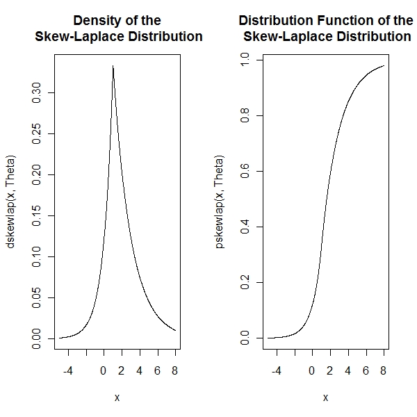
> curve(dskewlap(x, Theta), from = -5, to = 8, n = 1000)
> title("Density of the\n Skew-Laplace Distribution")
> curve(pskewlap(x, Theta), from = -5, to = 8, n = 1000)
> title("Distribution Function of the\n Skew-Laplace Distribution") |
> dataVector <- rskewlap(500, Theta)
> curve(dskewlap(x, Theta), range(dataVector)[1], range(dataVector)[2],
+ n = 500)
> hist(dataVector, freq = FALSE, add = TRUE)
> title("Density and Histogram\n of the Skew-Laplace Distribution")
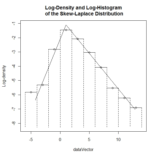
> logHist(dataVector, main = "Log-Density and Log-Histogram\n of the Skew-Laplace Distribution")
> curve(log(dskewlap(x, Theta)), add = TRUE, range(dataVector)[1],
+ range(dataVector)[2], n = 500) |
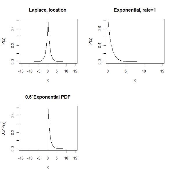
Using the library VGAM package .Laplace Distribution
> library(VGAM) > par(mfrow = c(2, 2)) > x1 <- seq(-15, 15, by = 0.05) > mylaplace1 <- dlaplace(x1, location = 0, scale = 1) > plot(x1, mylaplace1, type = "l", xlab = "x", ylab = "P(x)", main = "Laplace, location") > x2 <- seq(0, 15, by = 0.05) > myexp1 <- dexp(x2, rate = 1) > plot(x2, myexp1, type = "l", xlab = "x", ylab = "P(x)", main = "Exponential, rate=1") > myexp2 <- 0.5 * dexp(x1, rate = 1) > plot(x1, myexp2, type = "l", xlab = "x", ylab = "0.5*P(x)", main = "0.5*Exponential PDF") |
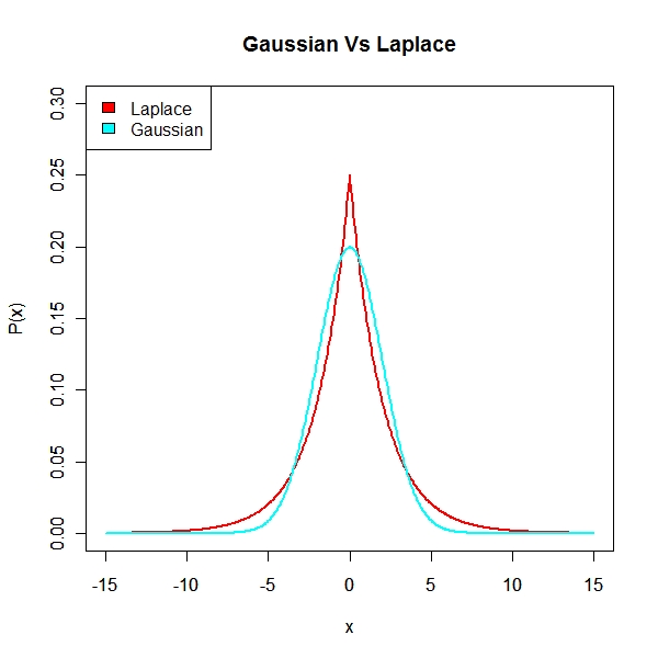
Compare Laplace Dist with Normal Dist
> library(VGAM)
> par(mfrow = c(1, 1))
> cols <- rainbow(2)
> x1 <- seq(-15, 15, by = 0.05)
> mylaplace1 <- dlaplace(x1, location = 0, scale = 2)
> plot(x1, mylaplace1, type = "l", xlab = "x", ylab = "P(x)", main = "Gaussian Vs Laplace",
+     lwd = 2, col = cols[1], ylim = c(0, 0.3))
> par(new = T)
> mynorm1 <- dnorm(x1, mean = 0, sd = 2)
> plot(x1, mynorm1, type = "l", xlab = "x", ylab = "P(x)", main = "",
+     lwd = 2, col = cols[2], ylim = c(0, 0.3))
> legend("topleft", legend = c("Laplace", "Gaussian"), fill = cols) |
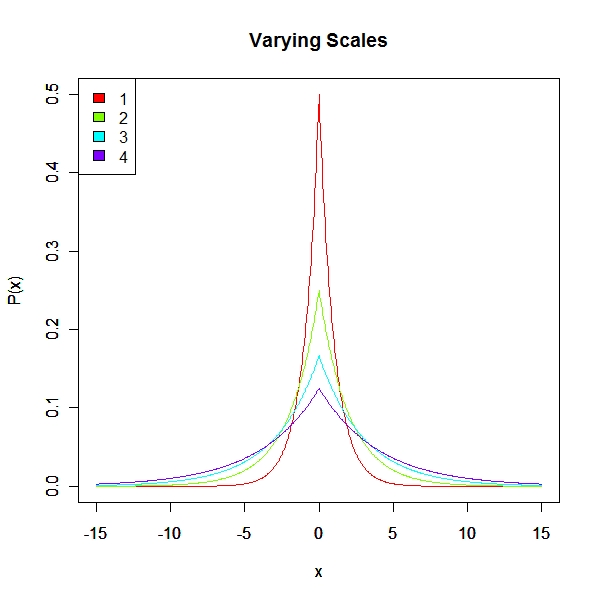
Scale Changes
> library(VGAM)
> par(mfrow = c(1, 1))
> cols <- rainbow(4)
> x1 <- seq(-15, 15, by = 0.05)
> mylaplace1 <- dlaplace(x1, location = 0, scale = 1)
> plot(x1, mylaplace1, type = "l", xlab = "x", ylab = "P(x)", main = "Varying Scales",
+     col = cols[1], ylim = c(0, 0.5))
> mylaplace1 <- dlaplace(x1, location = 0, scale = 2)
> par(new = T)
> plot(x1, mylaplace1, type = "l", xlab = "x", ylab = "P(x)", main = "",
+     col = cols[2], ylim = c(0, 0.5))
> mylaplace1 <- dlaplace(x1, location = 0, scale = 3)
> par(new = T)
> plot(x1, mylaplace1, type = "l", xlab = "x", ylab = "P(x)", main = "",
+     col = cols[3], ylim = c(0, 0.5))
> mylaplace1 <- dlaplace(x1, location = 0, scale = 4)
> par(new = T)
> plot(x1, mylaplace1, type = "l", xlab = "x", ylab = "P(x)", main = "",
+     col = cols[4], ylim = c(0, 0.5))
> legend("topleft", legend = 1:4, fill = cols) |
Location Changes
> par(mfrow = c(1, 1))
> cols <- rainbow(4)
> x1 <- seq(-15, 15, by = 0.05)
> mylaplace1 <- dlaplace(x1, location = 0, scale = 1)
> plot(x1, mylaplace1, type = "l", xlab = "x", ylab = "P(x)", main = "Varying Locations",
+     col = cols[1], ylim = c(0, 0.5))
> mylaplace1 <- dlaplace(x1, location = 1, scale = 1)
> par(new = T)
> plot(x1, mylaplace1, type = "l", xlab = "x", ylab = "P(x)", main = "",
+     col = cols[2], ylim = c(0, 0.5))
> mylaplace1 <- dlaplace(x1, location = 2, scale = 1)
> par(new = T)
> plot(x1, mylaplace1, type = "l", xlab = "x", ylab = "P(x)", main = "",
+     col = cols[3], ylim = c(0, 0.5))
> mylaplace1 <- dlaplace(x1, location = 3, scale = 1)
> par(new = T)
> plot(x1, mylaplace1, type = "l", xlab = "x", ylab = "P(x)", main = "",
+     col = cols[4], ylim = c(0, 0.5))
> legend("topleft", legend = 1:4, fill = cols) |