Non Central Chi-Square - Chap 7

Purpose
To explore Chi Square distribution.

Non Central Chi Square Distribution

> library(mnormt)
> nc <- 100
> nr <- 10000
> sample.data <- matrix(data = NA, nrow = nr, ncol = nc)
> for (i in seq_along(sample.data[1, ])) {
+     sample.data[, i] <- rnorm(nr)
+ }
> sample.data <- t(sample.data)
> sample.data <- sample.data + 2
> sample.data <- sample.data^2

Summary Stats

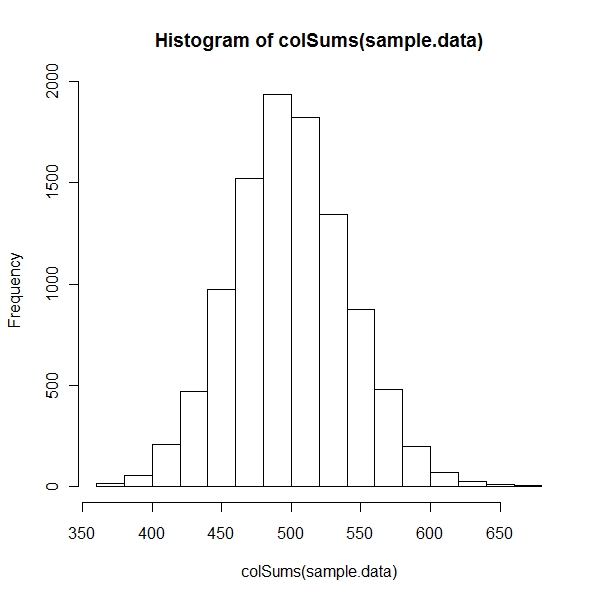
> mean(colSums(sample.data))
[1] 499.334
> var(colSums(sample.data))
[1] 1754.506

Histogram of a non central chi square distribution

> hist(colSums(sample.data))

Non central chi square in R

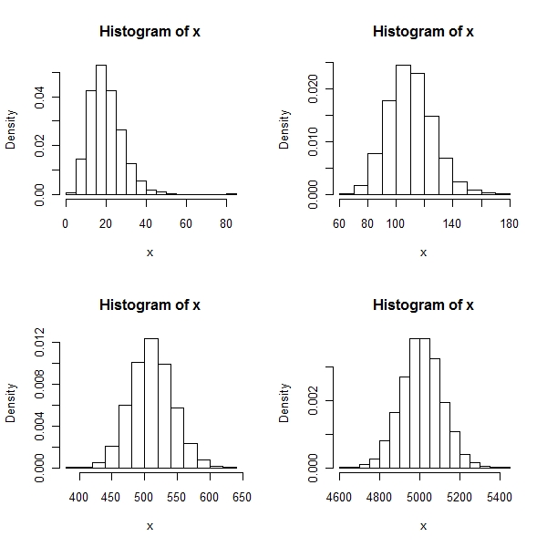
> par(mfrow = c(2, 2))
> x <- rchisq(n = nr, df = 10, ncp = 10)
> hist(x, prob = T)
> x <- rchisq(n = nr, df = 100, ncp = 10)
> hist(x, prob = T)
> x <- rchisq(n = nr, df = 500, ncp = 10)
> hist(x, prob = T)
> x <- rchisq(n = nr, df = 5000, ncp = 10)
> hist(x, prob = T)

> par(mfrow = c(2, 2))
> x <- rchisq(n = nr, df = 10, ncp = 10)
> qqnorm(x)
> x <- rchisq(n = nr, df = 100, ncp = 10)
> qqnorm(x)
> x <- rchisq(n = nr, df = 500, ncp = 10)
> qqnorm(x)
> x <- rchisq(n = nr, df = 5000, ncp = 10)
> qqnorm(x)

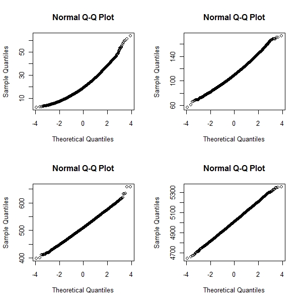
As degrees of freedom increase, the more it becomes like normal

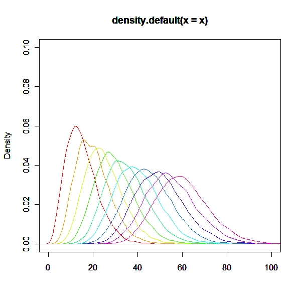
> par(mfrow = c(1, 1))
> plot.new()
> cols <- rainbow(10)
> for (i in 1:10) {
+     par(new = T)
+     x <- rchisq(n = nr, df = 5 * i, ncp = 10)
+     plot(density(x), col = cols[i], xlim = c(0, 100), ylim = c(0,
+         0.1), xlab = "")
+ }